Documents

Ocean Mesoscale, Sub-mesoscale, and Internal Wave Variability and Dynamics

Roger M. Samelson (Oregon State University), Dudley B. Chelton (Oregon State University), J. Thomas Farrar (Woods Hole Oceanographic Institution), M. Jeroen Molemaker (University of California, Los Angeles)

1. Introduction & Objectives

The overall project goals are to assess how oceanic mesoscale, sub-mesoscale, and internal wave signals may be manifest in SWOT measurements and how to use SWOT data to develop new physical insight into these phenomena, and to contribute to addressing the associated challenges posed to the SWOT mission. Specifically, the planned work will include: (1) characterizing internal wave SSH signals relevant to SWOT and exploring approaches for filtering these signals to remove or reduce internal-wave contamination of the SSH signals associated with mesoscale and sub-mesoscale motions that are the focus of the SWOT mission; (2) evaluating the potential of noisy SWOT SSH data for estimation of mesoscale/sub-mesoscale vertical velocity from extended Ekman theory and internal balanced dynamics (following QG, SQG, and other theory); and (3) evaluating the potential of SWOT SSH data for understanding mesoscale/sub-mesoscale geostrophic dynamics. Consideration of sampling patterns, for both the fast-repeat and 21-day repeat orbits, will be essential especially in the later phases of the project. The work will include a regional focus on the California Current System (CCS) region.

Following Klein et al. (2015), sub-inertial ocean variability may be divided into the "mesoscale," corresponding to wavelengths greater than 50 km, and the "sub-mesoscale," corresponding to wavelengths less than 50 km. The primary oceanographic objective of the SWOT mission as expressed in the SWOT SRD (Rodriguez, 2015) and OBP ATBD (Peral 2014) is to enable study of mesoscale and sub-mesoscale eddies, fronts, and filaments on wavelength scales down to about 10 km, which are inaccessible with previous satellite altimeters and difficult to observe with in situ measurements. A notional extension of a global-mean wavenumber power-spectrum of SSH from existing nadir altimeter data (Fu and Ubelmann 2014) is used in the SWOT SRD and OBP ATBD documents to illustrate anticipated SWOT measurement capabilities (Fig. 1). The high-wavenumber (short-wavelength) extrapolation remains above the expected noise floor of SWOT measurements down to wavelengths of about 10 km. However, the noise requirements for SWOT and their dependence on resolution and smoothing are complicated by the 2-dimensional (2-d) swath measurement and the anticipated spatio-temporal inhomogeneity of the noise. Because few direct observations of horizontal wavenumber spectra of internal-wave, small-mesoscale and sub-mesoscale SSH variability are available, and because of the complexity of the SWOT noise and sampling patterns, a substantial part of our planned research is directed at quantifying the relevant oceanographic signals in the context of SWOT, in order to provide a basis for future filtering strategies and to determine the implications of the results for SWOT prelaunch planning and scientific development.

Fig. 1 — Figure 1. 1-sided, 1-d wavenumber spectra of SWOT baseline science requirements for measurement errors before (blue solid line) and after (red solid) 2-d smoothing of the OBP SSH data to eliminate variance at wavelengths shorter than 15 km. The SRD noise requirement (red solid) is the sum of the red (orbit error and long-wavelength measurement error) noise (dotted red) and white (residual uncorrelated error) noise that has been smoothed with an idealized filter having magnitudes of 1 for wavelengths longer than 15 km and 0 for shorter wavelengths (dashed red). The noise requirement [derived in Chelton et al. (2015)] for the 1‐km OBP data (solid blue) is the sum of the red noise (dotted red) and the white noise in the OBP data (dashed blue). For comparison, the mean (black) and 68 percentile (cyan) SSH spectra from the SRD and OBP ATBD and the existing nadir-altimeter [Jason-1,2; from Fu and Ubelmann (2014)] noise floor (purple) are also shown. This figure is a modified version of Figs. 1 of the SRD and OBP ATBD.

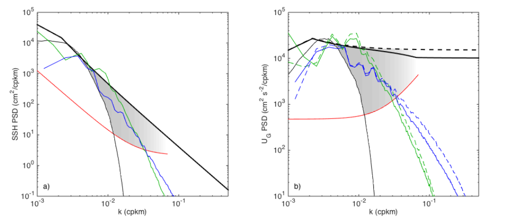
Comparison of 1-d SSH spectra computed from the AVISO 2-d mapped dataset (Ducet et al., 2000) with the SRD SSH spectrum illustrates the new SSH information potentially available from SWOT mission observations for mesoscale/sub-mesoscale studies (Fig. 2a). In the 1-d 2 spectral description (Fig. 2), the new SSH information that SWOT will potentially provide for mesoscale/sub-mesoscale studies is represented by an approximately triangular region of spectral variance (Fig. 2a, shaded area). Numerical simulations suggest the existence of an approximate power-law dependence of SSH and velocity spectral densities from the mesoscale into the submesoscale range; different models, however, produce different spectral slopes. The shallow, approximately k^-2 slope of the SRD SSH spectrum implies a nearly flat spectrum for cross-track geostrophic velocity, if the latter is inferred directly from the SSH gradient. Such a flat velocity spectrum implies mean velocity variances of order 103 cm² s^-2 in the sub-mesoscale range, which may be unrealistically large, as illustrated by comparison of model velocity spectra with the inferred SRD geostrophic velocity spectrum (Fig. 2b). Ocean spectral energy levels in the submesoscale range are unknown and additionally will vary temporally and between geographic regimes. Nonetheless, one interpretation of this difference in velocity spectral levels (Fig. 2b) is that internal-wave and related high-frequency processes may contribute substantially to the SSH spectrum in the sub-mesoscale range, and thus to the practical resolution limits for SWOT studies of mesoscale/sub-mesoscale variability.

Fig. 2 — Figure 2. 1-dimensional (1-d) spectra for (a) SSH and (b) "cross-track" velocity, with the regions of new mesoscale/sub-mesoscale variance accessible from SWOT indicated (gray shading). (a) The SRD notional SSH mean spectrum (in simplified form; thick black solid line) and SWOT noise requirement for 15-km smoothing (red) from Fig. 1; the mean of zonal 1-d SSH spectra computed by Chelton et al. (2011; Fig. A3a) from the AVISO 2-d mapped dataset (thin black); and 1-d SSH spectra from numerical simulations (CCS1: blue; CCS2: green). (b) 1-d spectra of: geostrophic estimates of cross-track velocity for the SRD (thick dashed black), AVISO (thin black), and SWOT noise requirement (red) obtained by multiplying the corresponding SSH spectra in (a) by g²k²f^-2 (for gravitational acceleration g and Coriolis parameter f ); model cross-track velocity (solid) and geostrophic cross-track velocity (dashed) for CCS1 (blue) and CCS2; illustrative SRD "balanced velocity" (solid black) obtained by correcting the SRD geostrophic velocity spectrum by a scaling that gives a rough quantitative estimate of the amplitude of the cyclostrophic bias discussed in the text.

2. Approach & Preliminary Results

Topic 1: Characterizing and Filtering/Isolating Internal Wave SSH Signals

We plan to focus on constructing quantitative observational estimates of the contribution of internal waves to SSH variability on the 15-100 km wavelength scales that SWOT will sample, primarily using mooring data, tide-gauge data, and high-resolution transect data (e.g, Farrar et al., 2007), along with theoretical considerations, to estimate the contribution of internal waves to the SSH wavenumber spectrum. We have made two different preliminary estimates of the contribution of internal waves to the SSH wavenumber spectrum. The first estimate uses mooring time series of dynamic height along with standard internal wave theory and reasonable assumptions (e.g., dynamic height signal dominated by 1^st baroclinic mode) to transform the internal-wave band of the frequency spectrum of dynamic height into a wavenumber spectrum and then, through basic modal theory (e.g., Farrar and Durland, 2012), into a wavenumber spectrum of SSH. These calculations suggest that the spatial variance of the SSH signatures of internal waves will be an order of magnitude larger than SWOT’s noise variance over wavelengths of 10-100 km, and may also exceed the variance of the submesoscale variability that SWOT is intended to observe (Fig. 3, top panels). The second estimate uses the ‘universal’ GM (Garrett-Munk; Garrett and Munk, 1972, 1975; Munk, 1981) internal-wave spectrum to construct a global, geographically varying, field of internal-wave SSH variance. For the global GM estimate (Fig. 3, bottom panel), we have expressed the result as the ratio of GM-based SSH variance to SWOT SRD baseline noise variance in the 15-100 km wavelength band (0.22 cm², or 0.47 cm standard deviation). The resulting estimated internal-wave SSH variance exceeds the noise variance essentially everywhere, in many regions by an order of magnitude.

Fig. 3 — Figure 3. Estimates of contributions of the internal-wave continuum to SSH spectral variance at wavelengths of 10-100 km. Top: SSH wavenumber spectra estimated from mooring data by converting dynamic height to SSH assuming the dynamic height is dominated by vertical mode 1 (blue lines); estimates from the Garrett-Munk internal wave spectrum (green lines). The SWOT noise spectra (red lines) are from the SRD and are the same as in Fig. 1. Lower panel: Global estimate of the ratio of internal-wave SSH variance to SWOT noise in the 15-100 km wavelength band; the assumptions going into the SSH estimate will be refined substantially as part of the proposed work.

Topic 2: Estimation of Mesoscale and Sub-mesoscale Vertical Velocity

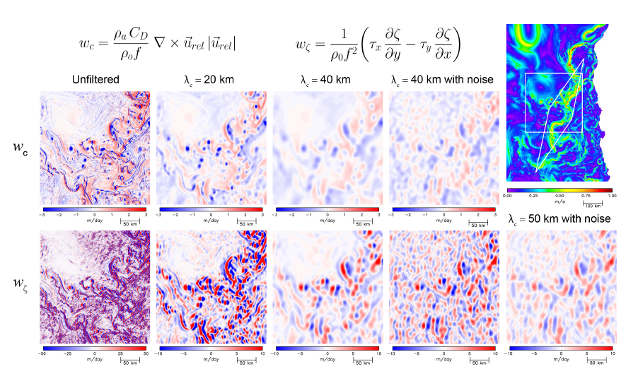
A novel and exciting aspect of the high-resolution SSH data from the planned SWOT mission involves its use to infer near-surface vertical velocity in the mesoscale and submesoscale regimes. Our research on the mesoscale and sub-mesoscale vertical velocity field will focus on two basic elements. The first consists of externally forced vertical motions induced by large-scale winds over mesoscale and sub-mesoscale features. The second consists of internaldynamical vertical motions associated with intrinsic, balanced evolution of the sub-inertial, near3 geostrophic variability. We have conducted a preliminary investigation of the effects of SWOT measurement errors on these estimates, using SSH fields from the CCS1 simulation. This analysis establishes the basic relevance of our proposed use of numerical simulations and illustrates both the potential value of SWOT observations and practical issues of the importance of smoothing of SWOT data in ground-based post-processing. With 40-km smoothing, the effects of 2.75 cm uncorrelated noise [the 1-km equivalent of the 15-km baseline SRD specification; see Fig. 1 and Chelton et al. (2015)] added to the model SSH field are readily apparent in geostrophic estimates of w_c and w_ζ (Fig. 4, 4^th column). When compared with the noise-free estimates (Fig. 4, 3rd column), it is apparent that w_c can be estimated reasonably well but that the w_ζ field is noisy. Increasing the smoothing to 50 km reduces the noise in the w_ζ field to a level that may be acceptable (Fig. 4, lower right). While such smoothing would be disappointing in view of the much more energetic variability at smaller scales, it should be kept in mind that our present understanding of w_c and w_ζ is limited to spatial scales larger than about 200 km and time scales longer than a month (Gaube et al., 2015).

Fig. 4 — Figure 4. Scale dependence of the two current-related components of Ekman pumping, and the effects of SWOT measurement errors. The equations at the top from Gaube et al. (2015) show that w_c depends on surface currents through relative wind (urel, air velocity minus surface current velocity) and w_ζ on the gradient of surface current vorticity. Upper right: snapshot of surface current speed in the 24° rotated coordinate system of the full CCS1 model domain with a white diamond overlaid to show the intersecting ascending and descending sampling swaths in the fast-sampling phase of the SWOT mission. The white square corresponds to the subdomain for which w_c and w_ζ are shown in the 1st and 2nd rows, respectively. Column 1: unfiltered w_c and w_ζ on the 0.5° model grid. Cols. 2-3: noise-free results after smoothing with half-power filter cutoff wavelengths of λc=20 and 40 km; note the different color bars for w_ζ. Col. 4: results with noise after smoothing with λc =40 km. Lower right: w_ζ with noise and λc =50 km smoothing.

Topic 3: Mesoscale and Sub-mesoscale Geostrophic Dynamics

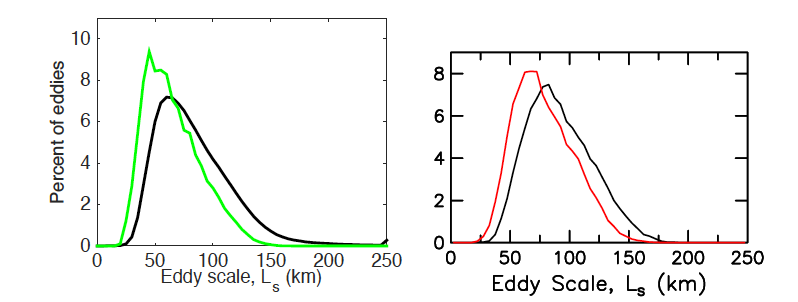
Chelton et al. (2011) have presented a comprehensive analysis of mesoscale eddies in the global ocean, based on the application of an SSH-based eddy tracking algorithm to the AVISO 2- d mapped dataset, and Samelson et al. (2014, 2016) have shown that a stochastic-field SSH model reproduces many of the observed eddy statistics. The high-resolution SSH observations to be obtained from the SWOT mission offer potential new opportunities to extend and improve this description of the oceanic eddy field, and to advance understanding of the associated dynamics. Our goal in this component of the planned research is to explore and define these potential contributions and their relation to SWOT mission requirements, in order to prepare for optimal scientific interpretation of the SWOT data when it becomes available. This work will necessarily rely primarily on model simulations, because these scales are not resolved by existing observations. Of particular relevance for SWOT are results relating to eddy horizontal scales, which are potentially affected by the resolution limits of the AVISO mapped data, and for which the high-resolution SWOT data promises to provide especially valuable improvements. The distribution of eddy length (radius) scales, from all weekly observations of globally tracked eddies with lifetimes of 16 weeks or greater, has a mean near 70 km (140-km eddy width) and is skewed toward large scales with an abrupt decrease for scales shorter than 50 km (Fig. 5a). Preliminary analysis of a high-resolution (1/10° grid) South Atlantic numerical simulation shows an eddy distribution similar to that observed for the same region, but shifted measurably toward smaller scales (Fig. 5b). This comparison suggests that many long-lived, smaller scale eddies are not captured by the mapped AVISO dataset because of its resolution limitations, but the scale cut-off near 25-50 km may also derive from dynamical constraints. We plan to conduct eddy identification and eddy dynamical analysis of numerical model simulations and stochastic-field SSH model simulations; and then to combine the results with focus on determining the space and time scales that must be resolved in order to make progress on understanding the physics of mesoscale eddy evolution. This work will then be extended to incorporate relevant results on noise and resolution limitations and to address the effects of various SWOT mission sampling configurations on the utility of SWOT data for (i) extension of eddy-tracking approaches to smaller horizontal spatial scales and (ii) dynamical analysis of mesoscale-eddy evolution events for eddies that would be of sufficiently large scale to be identified (but not dynamically analyzed) in the current merged altimeter dataset.

Fig. 5 — Figure 5. Tracked eddy length (radius, or half-width) scale distributions for eddies with lifetimes of 16 weeks or greater. (a: left panel) global AVISO (black) and stochastic model (green); (b: right) South Atlantic AVISO (black) and South Atlantic model simulation (red).

References

Chelton, D.B., M.G. Schlax, and R.M. Samelson, 2011. Global observations of nonlinear mesoscale eddies. Progress Oceanogr., 91, 167-216.

Chelton, D.B., R.M. Samelson, and J.T. Farrar, 2015. Theoretical Basis for the Resolution and Noise of SWOT Estimates of Sea-Surface Height. Unpublished manuscript. Available for download at: http://www-po.coas.oregonstate.edu/~rms/ocean/.

Ducet, N., Le Traon, P.-Y., Reverdin, G., 2000. Global high resolution mapping of ocean circulation from TOPEX/POSEIDON and ERS-1/2. J. Geophys. Res. 105, 19477–19498.

Farrar, J.T., C. Zappa, R. A.Weller, and A.T. Jessup, 2007. Sea surface temperature signatures of oceanic internal waves in low winds. Journal of Geophys. Res., 112, C06014, doi:10.1029/2006JC003947.

Farrar, J.T., and T.S. Durland, 2012. Wavenumber-frequency spectra of inertia-gravity and mixed Rossby-gravity waves in the equatorial Pacific Ocean. J. Phys. Oceanogr., 42, 1859–1881. Farrar, J.T., Chelton, D.B., Samelson, R. and Durland, T.S. How will oceanic internal waves appear in SWOT data? SWOT Science Definition Team Meeting, Pasadena, CA, 2013.

Fu, L.-L., and C. Ubelmann, 2014. On the transition from profile altimeter to swath altimeter for observing global ocean surface topography. J. Atmos. Oceanic Technol., 31, 560-568.

Garrett, C.J.R., and W.H. Munk, 1972. Space‐timescales of internal waves, Geophys. Fluid. Dyn., 2, 225–264.

Garrett, C.J.R., and W.H. Munk, 1975. Space‐timescales of internal waves. A progress report, J. Geophys. Res., 80, 291–297.

Gaube, P., D.B. Chelton, R.M. Samelson, M.G. Schlax and L.W. O'Neill, 2015: Satellite observations of mesoscale eddy-induced Ekman pumping. J. Phys. Oceanogr., 45, 104- 132.

Klein, P.J., and Co-Authors, 2015. Mesoscale/sub-mesoscale dynamics in the upper ocean. SWOT SDT White Paper. Available at: http://swot.jpl.nasa.gov/science/resources/.

Munk, W. ,1981. Internal waves and small‐scale processes, in Evolution of Physical Oceanography, edited by B. A. Warren and C. Wunsch, pp. 264–291, MIT Press, Cambridge, Mass.

Peral, E., 2014: KaRIn: Ka-band Radar Interferometer On-Board Processor (OBP) Algorithm Theoretical Basis Document (ATBD). Jet Propulsion Laboratory document JPL D-79130, Draft Release, November 21, 2014.

Rodriguez, E., 2015: Surface Water and Ocean Topography Mission (SWOT) Project Science Requirements Document. Jet Propulsion Laboratory document JPL D-61923, Initial Release, February 12, 2015.

Samelson, R.M., M.G. Schlax, and D.B. Chelton, 2014. Randomness, symmetry, and scaling of mesoscale eddy lifecycles. J. Phys. Oceanogr., 44, 1012–1029, doi: 10.1175/JPO-D-13-0161.1; corrigendum doi: http://dx.doi.org/10.1175/JPO-D-14-0139.1.

Samelson, R.M., M.G. Schlax, and D.B. Chelton, 2016. A linear stochastic field model of mid-latitude mesoscale sea-surface height.