Water Level and Discharge Estimation with a Polynomial Surrogate Model for Uncertainty Quantification and Data Assimilation - Application to a Real Test Case: The Garonne Valley

Contribution of the CECI1 (CERFACS/CNRS, France) – LNHE2 (EDF R&D, France) Group to the SWOT Mission

S. Ricci (CECI, CERFACS/CNRS - France), N. Goutal (EDF/LNHE/Laboratoire - France), N. El Mocayd (CECI, CERFACS/CNRS - France)

1. Introduction & Objectives

The group is composed of CECI (CERFACS/CNRS, Toulouse, France) and LNHE (EDF R&D, Chatou, France). It gathers expertise in hydraulic modeling (TELEMAC-MASCARET software) and applied mathematics with a focus on uncertainty quantification (UQ) (sampling, analysis of variance, surrogate models) and data assimilation (DA) (ensemble-based methods, filtering algorithms, variational methods). The group has been working together for several years; the most significant developments stand in the implementation of Kalman Filter derived algorithm for model state and parameters correction via DA of in-situ observations and its operational use for flood forecasting and water resource management. A perspective for these studies, developed here, is to use Surface Water and Ocean Topography (SWOT) data to improve hydraulic model parameters and results and consequently improve water level and discharge simulation and forecast.

The predictive capability of free surface flow hydrodynamic models is limited by uncertainties in the description of data (initial conditions – boundary conditions – river geometry) and physical parameters (friction coefficient). UQ methods are largely used for Sensibility Analysis (SA) to estimate how and how much uncertainties in the inputs translate into errors in simulated water level and discharge. Once identified, these uncertainties can be reduced with DA algorithms. In the context of ensemble based methods and large amount of assimilated data such as that from the Surface Water and Ocean Topography (SWOT) mission, the cost of the UQ study and DA algorithm should be reduced. A Polynomial Chaos (PC) surrogate model was implemented for MASCARET and validated over the Garonne river (France). It was then used for SA and to stochastically estimate the background error covariance matrix at a lower cost than that of classical Monte- Carlo approach. It was shown that with this PC-EnKF DA, the assimilation of synthetical SWOT data allows for the correction of the water level and discharge.

2. Methodology

2.1 Hydraulic Modeling

MASCARET [1] is an open-source software developed by EDF R&D and CEREMA (http://www.opentelemac.org). It solves the one-dimensional Shallow Water Equations (SWE) [2] that are derived from two prime principles: mass conservation (Eq. 1) and momentum conservation (Eq. 2) written in terms of hydraulic section A(x,t) and discharge q(x,t).

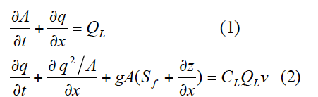
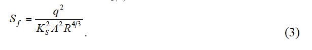
where x is the curvilinear abscissa along the hydraulic axis of the reach, z(x,t) is the water surface elevation, Q_L(x,t) is the lateral discharge, C_L(x,t) is the lateral discharge coefficient, v(x,t) = q/A is the mean velocity and S_f is the friction term that depends on the Strickler coefficient K_s(x):

2.2 Polynomial Chaos Surrogate Model

The formulation of the Polynomial Chaos (PC) surrogate ([3], [4], [5], [6]) is presented for n random variables included in the random vector x. The Strickler coefficient K_s and the constant river discharge Q (steady flow) are known to be the most relevant sources of uncertainty in water level predictions and are thus included in the random vector X. In the following, details are given on the methods used to compute the PC coefficients (truncation strategy, projection strategy, choice of polynomial basis), derive the statistics of the water level h and evaluate the accuracy of the PC surrogate.

The input random variables are supposed to be independent with finite variance and defined in a proper probabilistic space. The random variables are casted in the random vector X = [x₁,...,x_n]^T, rescaled in the standard probabilistic space (0 mean and unit variance) and denoted by ξ to which PC framework applies. The physical model M maps x onto the output space to formulate the spatially distributed water level in the river, this vector is assumed to be of finite variance. Thus for each curvilinear abscissa or cross-section, h can be projected onto a stochastic space spanned by orthogonal polynomial functions:

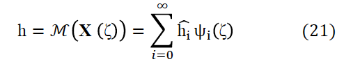
here (ψ_i) with (i = 0,...,∞) designate the multi-variate polynomial functions that are defined as orthogonal with respect to the joint density of x, where i is the multi-index identifying the polynomial components in the multi-variate space, and where h_i are the corresponding deterministic coefficients (or modes). This sum is truncated to a finite number of terms N_pc associated to the maximum polynomial order P and the number of random variables: N_pc = (n+p!)/n!p!. According to the Askey scheme, the Hermite polynomials form the optimal basis for random variables following a Gaussian distribution, and the Legendre polynomials are the counterpart for the uniform distribution [7]. In practice, the orthonormal basis is built using the tensor product of one-dimensional polynomial functions.

A non-intrusive spectral projection method is applied to compute the decomposition coefficients. It relies on the orthogonality property of the polynomial basis. In this framework, the i^th PC coefficient hi is computed as h_i = < h,ψ_i (ζ) > that involves the computation of an integral estimated through a standard Gaussian quadrature rule:

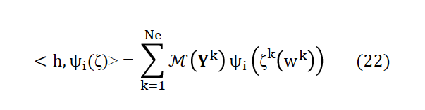
where h^(k) = M(Y^k) corresponds to the direct model integration evaluated at the k^th quadrature root Y^k = [Q^k, K_s^k] (in the physical space) with its associated weight w_k. Here k varies between 1 and N_e, with N_e = (N_quad)ⁿ when N_quad quadrature points are selected for each input random variable. The spectral projection strategy is thus achieved over an evaluation sample E_quad of size (N_quad)ⁿ. In order to guarantee that a polynomial function can properly be represented by the PC expansion, N_quad should be constrained by the total polynomial degree P such that: N_quad > P+1.

The spectral projection strategy proceeds as follows:

• Choose the maximum polynomial order P.
• Choose the number of quadrature roots N_quad per stochastic dimension and identify the roots in the normalized space.
• Map the normalized roots onto the physical space to formulate the quadrature roots vector Y = [y(1),..., y(N_quadⁿ)]^T, thus defining the input evaluation sample set E_quad.
• Integrate the direct model for the quadrature roots Y and formulate the output vector H = [h(1),...,h(N_quadⁿ)]^T.
• Compute the PC coefficient h_i with (i = 0,...,N_pc-1) and formulate M_pc.

The accuracy of the PC surrogate is evaluated in L₂ norm with respect to an independent sample E_mc of size N_mc = 10⁵ in the coefficients space and in the water level space. The water level Probability Density Function (PDF), its statistical moments, the covariance matrix for the water level along the cross sections and the Sobol indices from the ANOVA approach [8] can be estimated stochastically from sampling of M_pc or analytically from the PC decomposition coefficients.

3 Experimental Settings

The study is carried out over a 50-km reach of the Garonne river between Tonneins (curvilinear abscissa s = 13 km), downstream of the confluence with the river Lot, and La Réole (curvilinear abscissa x = 62 km), with an observing station at Marmande (x = 36 km). The mean slope over the reach is S₀ = 3.3 m.km^-1 and the mean width of the river is W = 250 m. The bank-full discharge is approximately equal to the mean annual discharge (Q = 1000 m³.s^-1). The hydraulic model for the Garonne River is built from 83 on-site bathymetry cross sections from which the full 1-D bathymetry is interpolated. The friction coefficient is spatially distributed over three homogeneous zones between Tonneins and x = 22 km, x = 22 km and Marmande and Marmande and La Réole. Despite the existence of active floodplains, this reach can be modeled accurately by a 1-D hydraulic model. For this test case, a single MASCARET integration for a typical flood event over 2 to 3 days takes about 30s CPU time. The main sources of uncertainty considered in the present work are (Q, Ks1, Ks2, Ks3); in the following, they are considered as physical random independent variables defined by their PDFs N(4031,400) for discharge and U(15; 60) for the three friction coefficients. With this choice of PDFs, the flow is subcritical because we consider only high flow conditions.

4 Results and Conclusions

A convergence study was carried out to identify the maximum polynomial order and the minimum number of quadrature points that are needed to formulate the surrogate model M_pc. The water level L₂ difference over sample E_mc was computed, it is of the order of 10^-4 for P = 6 and N_quad = 7. For the surrogate, the error on the mean and the variance is around 10^-6 and 10^-4 respectively. Figure 1-a compares the PDF in the upstream part of the Garonne reach (x = 22 km) of the Garonne reach obtained with a Monte-Carlo approach over E_mc (blue line) as well as with the surrogates mode M_pc (with P = 6 and N_quad = 7 in green, P = 15 and N_quad = 16 in red). Figure 1b presents the counterpart of Figure 1a at Marmande cross section (x = 36 km).

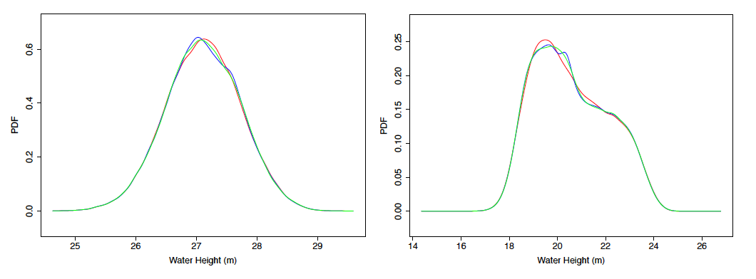
Figure 2a display the Sobol indices with respect to Q and K_s3 along the curvilinear abscissa computed with the polynomial surrogate model (P = 6, N_quad = 7). In the upstream part of the river, the bathymetry is quite smooth, the flow dynamic represented by the surrogate is driven by Q with S_q = 0.9 and S_Ks3 = 0.1. The relation between water level and discharge is fairly linear so that the water level PDF is almost Gaussian. A PC expansion of total degree P = 6 thus provides a satisfying description of the PDF upstream the Garonne reach. At Marmande cross section and in its neighboring, the error in water level in dominated by the error in K_s3 with S_q = 0.15 and S_Ks3 = 0.85. The flow dynamics is more complex since the bathymetry and the river width vary, the nonlinearities are stronger and the estimation of the PDF requires a higher total degree P (here P = 15) for the PC expansion.

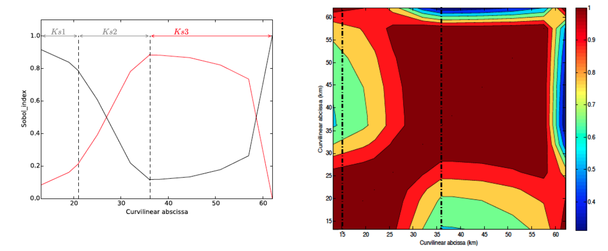
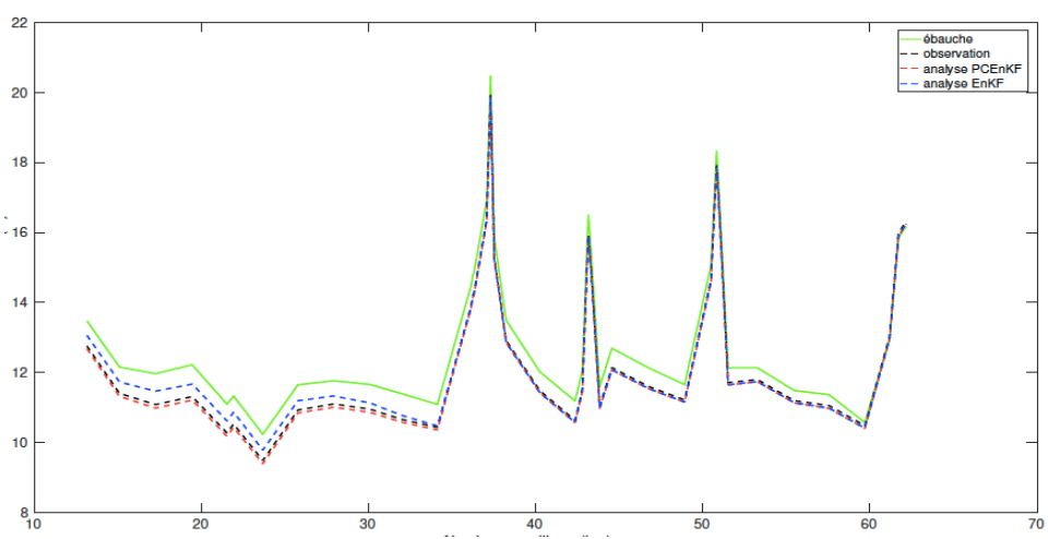
In the context of DA, the formulation of the Kalman gain matrix relies on the estimation of the water level error covariance matrix that describes the spatial correlation between the errors along the river cross sections. The use of the PC surrogate model in place of the direct model allows for a significant cost reduction for stochastic estimate of these statistics, which are here formulated using the PC coefficients directly. Figure 2b displays the water level correlation matrix along the 60-km Garonne reach that is estimated using the surrogate M_pc (P = 6, N_quad = 7) with respect to Q and K_s3. Two cross sections on the river are marked by vertical dashed lines at x = 22 km and x = 36 km. By definition, the correlation is equal to 1 at the location points where the correlations are expressed and decreases when moving to the other grid points along the channel. The correlation function for the upstream location x = 22 km displays large correlations over the area where the flow is dominated by the variability in Q. The correlation function for Marmande (x = 36 km), displays large correlations over Marmande neighboring where the flow is dominated by the variability in K_s3. It should be noted (not shown) that these correlations are estimated with an error on the order of 10^-7 with respect to those estimated with a classical Monte-Carlo approach based on E_mc (N_mc = 10⁵ evaluations of the direct model). In the EnKF, the correlation matrix evolves over time to represent the spatially-distributed and temporally-dependent patterns. Estimating this correlation matrix through the use of a PC surrogate (using only 49 direct model evaluations of the water level) is thus a promising approach to reduce the cost of the EnKF, while representing the correlations with satisfying accuracy. It was indeed used for PC-EnKF analysis illustrated in Figure 3 for an Observing System Synthetical Experiment where SWOT-like observations are generated from a reference model integration, at every simulation grid point. The observation error is described by a standard deviation of 10 cm. The assimilation is carried out every 4 days, it is here illustrated at a given time step and the current analysis is then used for forecast. The stochastic covariance estimation in EnKF is done with 49 forward model integration, similarly to the PC-EnKF. It appears that the EnKF is not converged contrary to the PC-EnKF and the PC-EnKF analysis is in better agreement with the observation then the EnKF. Additional results can be found in [8].

The perspective for this work is to extend the PC-strategy to unsteady flows and identify how often the surrogate model should be re-computed according to the time scales of the flow dynamics. Most importantly, this analysis should be carried out with realistic SWOT-like observations that result from the use of the SWOT-HR simulator.

Acknowledgements

The PhD grants of Nabil El Mocayd has been funded respectively by CNES & EDF. The authors acknowledge M. Baudin, S; Boyaval, A. Dutfoy, A.-L. Popelin, G. Blatman and B. Iooss from MRI (EDF R&D) for helpful discussions on uncertainty quantification and support on OpenTURNS.

References

[1] Goutal, N., Lacombe, J.-M., Zaoui, F., and El-Kadi-Abderrezzak, K. (2012). MASCARET: a 1-D open-source software for flow hydrodynamic and water quality in open channel networks, River flow 2012, 1169- 1174.

[2] Hervouet, J.M. (2003). Hydrodynamique des écoulements à surface libre : Modélisation numérique avec la méthode des éléments finis. Presse de l'Ecole Nationale des Ponts et Chaussées.

[3] Le Maitre, O. and Knio, O. (2010). Spectral Methods for Uncertainty Quantification. Springer.

[4] Spanos, P. and Ghanem, R. (1991). Stochastic Finite Elements: A Spectral Approach. Springer.

[5] Xiu, D. (2010). Numerical Methods for Stochastic Computations: A Spectral Method Approach. Princeton University Press.

[6] Sudret, B. (2007). Uncertainty propagation and sensitivity analysis in mechanical models. Contributions to structural reliability and stochastic spectral methods. Accreditation to supervise research report.

[7] Xiu, D. and Karniadakis, G.E. (2002). The Wiener-Askey polynomial chaos for stochastic differential equations. SIAM Journal on Scientific Computing, 24-2, 619-644.

[8] Saltelli, A. (2002). Making best use of model evaluations to compute sensitivity indices. Computer Physics Communications. 145, 280-297.

[9] El Mocayd, N. (2017). La Décomposition en polynôme du chaos pour l'amélioration de l'assimilation de données ensembliste en hydraulique fluviale. PhD Université de Toulouse, INP.