Documents

Transition Scale from Geostrophic Flows to Wave Motions in the World Ocean

Project Title: Exploring New Upper Ocean Circulation Dynamics through Synergy of the SWOT Satellite Mission and High-Resolution OGCMs

B. Qiu (Department of Oceanography, University of Hawaii at Manoa - Honolulu, Hawaii, USA), S. Chen (Department of Oceanography, University of Hawaii at Manoa - Honolulu, Hawaii, USA), P. Klein (Laboratoire de Physique des Oceans, Ifremer/CNRS/UBO/IRD - Plouzane, France), J. Wang (Jet Propulsion Laboratory, California Institute of Technology - Pasadena, California, USA), L.-L. Fu (Jet Propulsion Laboratory, California Institute of Technology - Pasadena, California, USA), D. Menemenlis (Jet Propulsion Laboratory, California Institute of Technology - Pasadena, California, USA)

Fig. 1 — Figure 1. Horizontal wavenumber-frequency distributions of surface eddy kinetic energy in the 500kmx500km box centered on (a) 37°N, 164°E and (b) 7°S, 164°E of the Pacific Ocean. Based on hourly MITgcm output of 10/01/2011-09/30/2012. Dashed white lines denote the inertial and tidal frequencies. Solid white lines denote the dispersion relation for internal gravity waves (IGWs) with 10 different vertical modes. Solid black lines denote the lower frequency boundary of either the IWG dispersion curve or the permissible tides. Dashed black lines denote the frequency of the 36-hour filter.

Introduction

Advent of nadir-looking satellite altimetry in the early 1990s has revolutionized our ability to measure with high precision the global sea surface height (SSH) field and to explore, through geostrophy, the upper ocean circulation dynamics. This exploration has significantly advanced our understanding of mesoscale eddy signals that have temporal and spatial scales of 50-200 days and 150-500km, respectively. With the radar interferometry, the next-generation Surface Water and Ocean Topography (SWOT) satellite will improve the measured SSH resolution down to the spectral wavelength of 15km, allowing us to investigate for the first time the upper ocean circulation variability at the submesoscale range on the global scale. With the balanced geostrophic flows weaken as k^-2 ~ k^-3, unbalanced wave motions, however, can overtake within the 10-200km meso-submesoscale range. For SWOT mission, it is critical to identify the length scale at which the geostrophic flow loses its dominance and is overtaken by the unbalanced wave motions, for which geostrophy is no longer valid.

The overall goals of our project as part of the SWOT Science Team are:

To aid SWOT mission science preparation by evaluating spatio-temporal variability of SSH and surface velocity signals from available repeat ship-board ADCP measurements and high-resolution OGCM output from 1/48° MITgcm (llc 4320).
To advance our understanding of new upper ocean dynamics at O(5-200km) scales by analyzing high-resolution OGCM output and ADCP data, with the goal to maximize SWOT's scientific return.

Repeat underway ADCP measurements have been conducted by Japan Meteorological Agency along the 137°E meridian from the coast of Japan to offshore of New Guinea over the past two decades. The measurement transect not only crosses a wide geographical range of the wind-driven tropical and subtropical gyres in the northwestern Pacific, but also traverses sub-regions with very different governing dynamics. By analyzing the 33 repeat surveys from 2004-2016, our recent analysis reveals that the transition scale Lt, which separates the dominance between the balanced geostrophic and unbalanced wave motions, depend sensitively on the energy level of local mesoscale eddy variability (Qiu et al. 2017; Nature Commun.). In the eddy-abundant western boundary current region of Kuroshio, Lt can be shorter than 15km, whereas Lt exceeds 200km along the path of relatively stable North Equatorial Current.

To extend this analysis of ours to the global ocean, we present here preliminary results based on the global high-resolution MITgcm output.

Fig. 2 — Figure 2. Distribution of KE-based Lt values estimated from (a) the dynamical delineation method and (b) the 36-hour filtering method. Estimation of Lt is done in a 500kmx500km grid using the KE wavenumber-frequency spectra shown in Figure 1. White contours denote the 3000m water depth.

Approach

Hourly SSH and surface velocity output from the state-of-the-art high-resolution MITgcm simulation. The MITgcm llc4320 model has a 1/48° horizontal resolution and 90 vertical levels (1m vertical resolution at surface and 30m down to 500m depth). It is forced by 6-hourly ERA-Interim atmospheric reanalysis, as well as by a synthetic surface pressure field consisting of 16 most dominant tidal constituents. For our analysis, we use the output from 1 October 2011 to 30 September 2012 (366 days).

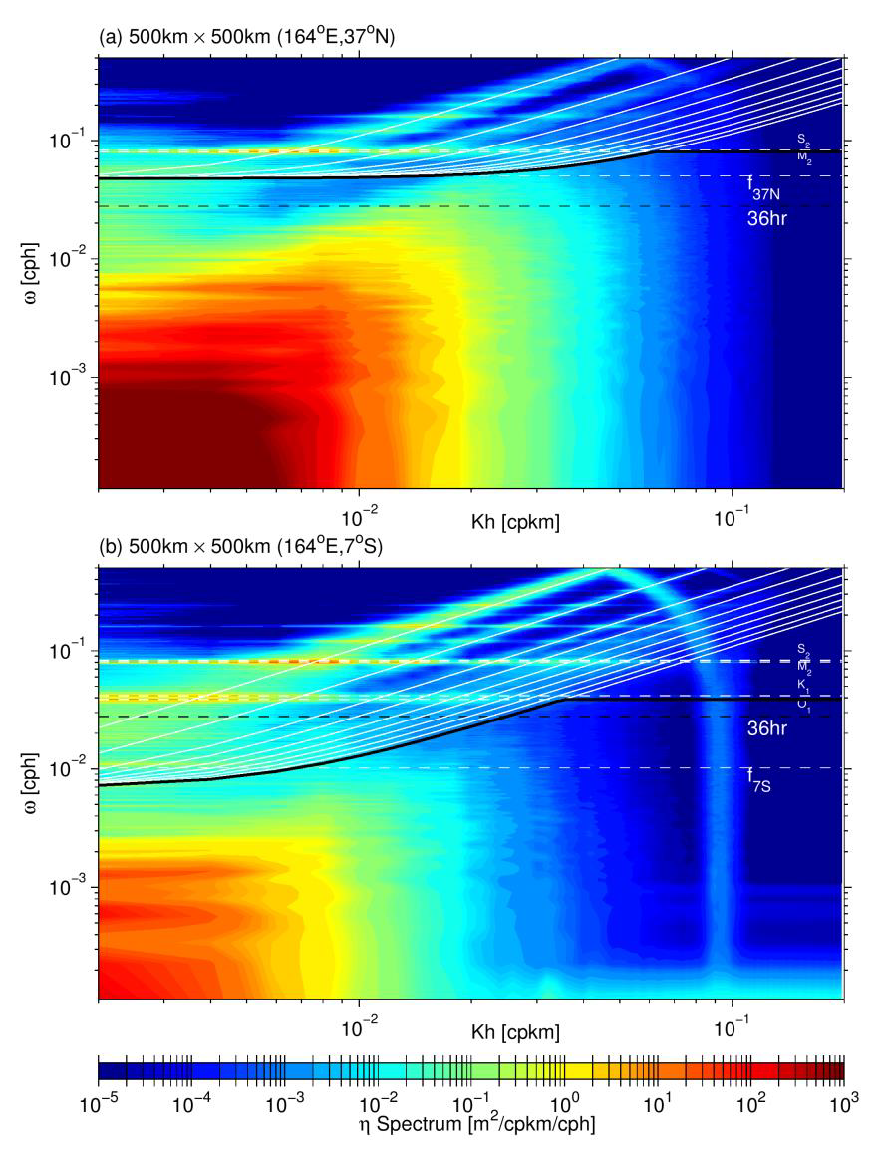
Delineation of balanced geostrophic and unbalanced wave motions can be conducted in several different ways. One commonly adopted method is to choose a temporal filter with the low-pass (high-pass) filtered signals regarded as geostrophic (wave) motions. For example, Richman et al. (2012; JGR) used a 48-hour filter in their study on kinetic energy (KE) spectral slopes of mesoscale eddies. Figure 1 compares the typical horizontal wavenumber-frequency spectrum of surface KE in the low-latitude (7°S) versus mid-latitude (37°N) Pacific Ocean from the MITgcm. From the plots, it is clear that the cutoff period delineating the balanced and wave motions is highly sensitive to the local inertial period. In fact, near the local inertial frequency band, balanced and wave motions can co-exist in different wavenumbers and this makes the adoption of a single cutoff filter undesirable. For the present study, we adopt a more dynamically-based method by defining the geostrophic (wave) motions below (above) the lower frequency of either the local internal-gravity-wave dispersion curve or the permissible tides (see black lines in Figure 1). The Lt variations based on this dynamical definition will be compared to those based on the traditional method with a 36-hour filter.

In addition to the transition scale Lt based on the surface KE spectra, we also estimate the Lt variations based on the SSH spectra from the hourly MITgcm output. In this latter case, Lt is defined as the spectral length scale at which the geostrophic SSH variance is equal to that of the unbalanced wave motions, either based on the dynamical delineation method or the 36-hour filtering method.

Analysis and Preliminary Results

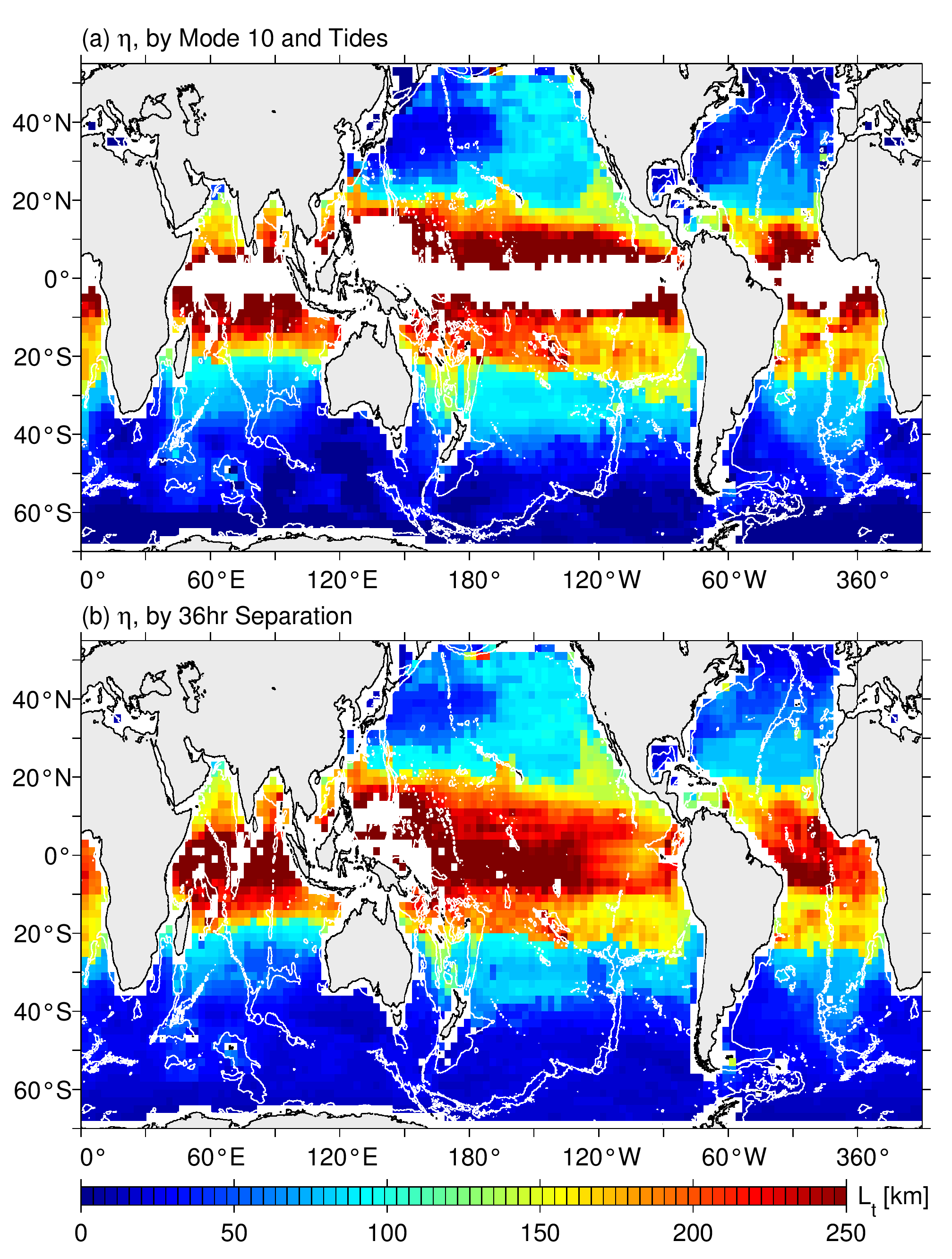
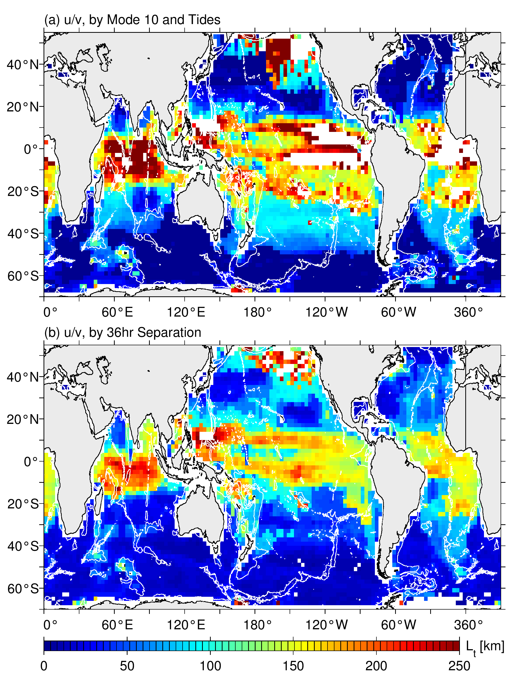
Fig. 3 — Figure 3. Distribution of SSH-based Lt values estimated from (a) the dynamical delineation method and (b) the 36-hour filtering method. Estimation of Lt is done in a 500kmx500km grid using the SSH wavenumber-frequency spectra. White contours denote the 3000m water depth.

Figure 2a shows the global KE-based Lt distribution using the dynamical delineation method. Consistent with the ship-board ADCP data results observed along 137°E in the northwestern Pacific (Qiu et al. 2017), Lt has the smallest value, < 50km, in the boundary current Kuroshio band south of Japan. It increases to ~100km in the weakly baroclinically-unstable Subtropical Countercurrent (STCC) band of 20°-30°N. The largest Lt is detected along the stable North Equatorial Current (NEC) band of 10°N where Lt exceeds 250km.

These results in the northwestern Pacific are typical for the rest of the global ocean. The Lt values smaller than 50km can be seen in all the western boundary current systems: the Kuroshio Extension, the Gulf Stream, the Agulhas Current, and the Brazil-Malvinas Confluence. The exception is in the East Australian Current (EAC) region and the reason for this will be commented on below. Also small in Lt is along the Antarctic Circumpolar Current (ACC) in the Southern Ocean, with the exceptions where prominent bottom topographic features exist, e.g., the Del Cano Rise, the Kerguelen Plateau, east of the Drake Passage, and around the southern end of the Mid-Atlantic Ridge. In most of the temperate latitudinal bands of 20°-30°, Lt falls in the O(100km) range. In the tropics equatorward of 15°, the Lt values often exceed 150km with the unbalanced motion signals overwhelming the balanced motion signals. In the extra-tropics, one area where Lt also exceed 150km is inside the Alaskan Gyre where oceanic mesoscale eddy variability is weak.

Compared to the Lt values estimated from the dynamical delineation method, Figure 2b shows the KE-based Lt distribution using the 36-hour filtering method. An overall and consistent difference between the two methods are (1) that Lt tends to be over-estimated in the mid- and high-latitude regions (with the exception in the Alaskan Gyre), and (2) that Lt tends to be under-estimated in the tropics in Figure 2b. This latitude-dependent bias is easy to understand because the 36-hour filter, as demonstrated in Figure 1a (1b), attributes some of the balanced (unbalanced) motion kinetic energy as that of the unbalanced (balanced) motion.

Figure 3 compares the global SSH-based Lt distributions using the dynamical delineation versus the 36-hour filtering method. The latitude-dependent differences between the two methods appear the same as those shown in Figure 2. At a fixed geographical location, the SSH-based Lt values are in general larger than the KE-based Lt values.

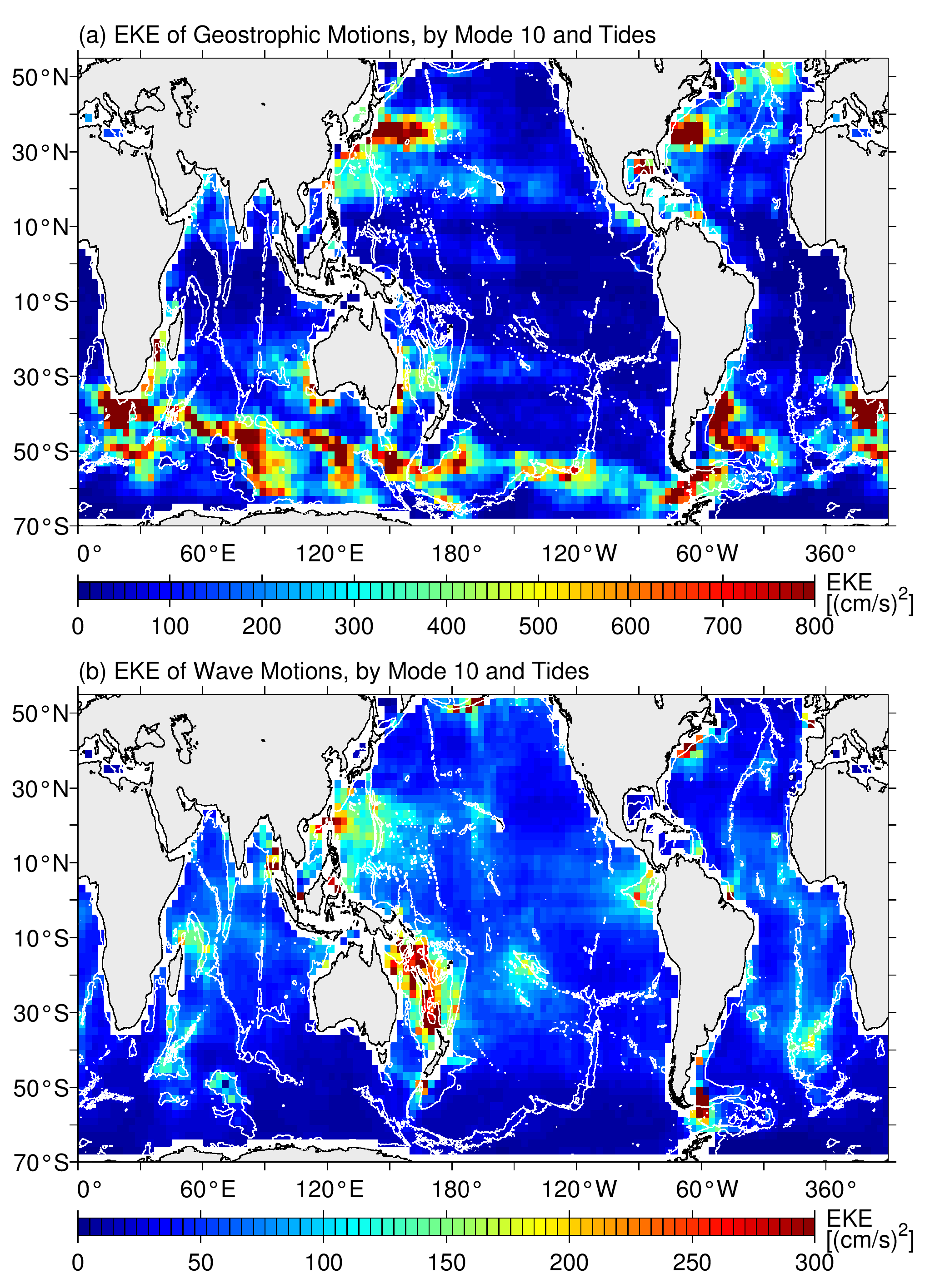
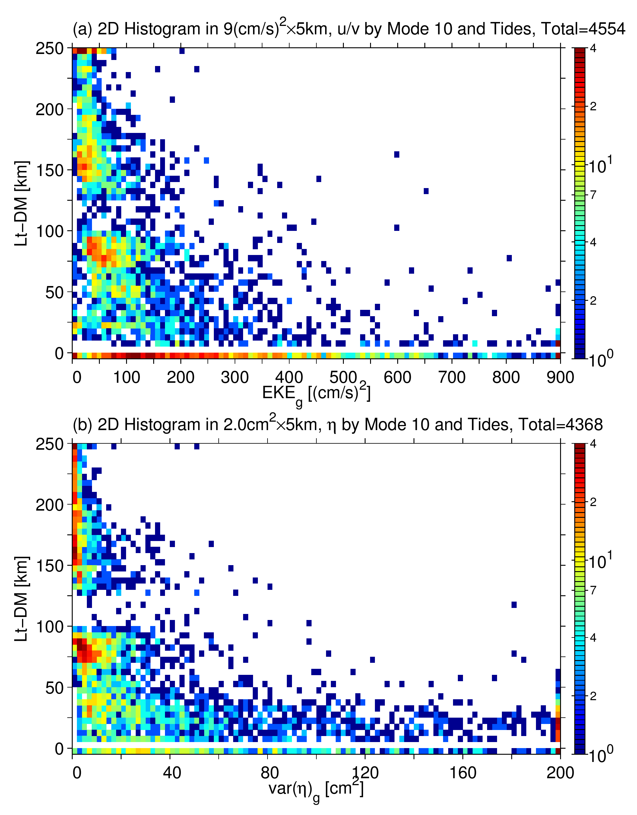
Fig. 4 — Figure 4. Distribution of surface eddy kinetic energy of (a) balanced geostrophic motions and (b) unbalanced wave motions based on the dynamical delineation method. Note that the color scales are different between (a) and (b). White contours denote the 3000m water depth.

That the Lt values are small in the western boundary current and ACC regions is not surprising because those are the regions in the world ocean with the largest balanced mesoscale eddy variability (see Figure 4a). It is, however, important to note that the level of mesoscale eddy variability is not the sole determinant for Lt. As indicated in Figure 5a that shows the histogram plot between Lt and the EKE level, despite the presence of a general inverse relationship, there exists much scattering between these two quantities. The reason for this is that the KE level for the unbalanced wave motions is geographically non-uniform. As shown in Figure 4b, the wave motion KE level is much higher in regions with prominent bottom topographic features, like the Philippine Sea in the northwestern Pacific and the Coral & Tasman Seas in the western South Pacific. In fact, it is this enhanced KE level associated with the unbalanced wave motions that is responsible for the large Lt values at 150-200km obtained in the Coral & Tasman Seas in Figure 2, despite the presence of the western boundary current EAC in the region.

Similar to the KE-based Lt case, the relationship for the SSH-based Lt values and the SSH variance for the balanced geostrophic motions (Figure 5b) is also complicated by the non-uniform global distribution of the SSH variance for the unbalanced wave motions. One interesting feature that is common in both Figs.5a and 5b, is that Lt has a two lope-sided distribution with a gap at 100-125km. At present, we are exploring dynamical reasons behind this and other features related to the global patterns of both EKE-based and SSH-based Lt values.

Fig. 5 — Figure 5. (a) Histogram of the balanced motion EKE and the KE-based Lt values based on the dynamical delineation method. The histogram is constructed using the 9.0cm²x5km bins. (b) Same as (a) except for the histogram of the balanced motion SSH variance and the SSH-based Lt values. The histogram is constructed using the 2.0cm²x5km bins.