Modeling Internal Wave Signals and their Predictability for SWOT

Brian K. Arbic (University of Michigan), Matthew H. Alford (University of California, San Diego), Maarten C. Buijsman (University of Southern Mississippi), Eric P. Chassignet (Center for Ocean-Atmospheric Prediction Studies, Florida State University), James B. Girton (Applied Physics Laboratory), Dimitris Menemenlis (NASA Jet Propulsion Laboratory), Hans E. Ngodock (Oceanography Division, Naval Research Laboratory), James G. Richman (Center for Ocean-Atmospheric Prediction Studies, Florida State University), Anna C. Savage (University of Michigan), Jay F. Shriver (Oceanography Division, Naval Research Laboratory), Xiaobiao Xu (Center for Ocean-Atmospheric Prediction Studies, Florida State University), Zhongxiang Zhao (Applied Physics Laboratory)

Abstract

We are working with high-resolution global simulations, of the HYbrid Coordinate Ocean Model (HYCOM) and the MITgcm, that are simultaneously forced by atmospheric and oceanic fields and that therefore resolve both mesoscale eddies and internal wave motions. We showed in Müller et al. (2015) that such models develop a partial spectrum of the internal gravity wave (IGW) continuum. Internal tides and the IGW continuum produce a high-frequency sea surface height (SSH) signal that will be temporally aliased in SWOT measurements. In our Science Team project we are investigating (1) the continuing improvement of internal tide maps empirically constructed from present-generation nadir altimeters, (2) the SSH wavenumber spectra of 1/50th degree North Atlantic HYCOM simulations of mesoscale eddies (without tides), (3) the incoherent internal tides, in particular the mechanisms underlying incoherence at the equator, (4) comparison of the modeled internal tides and waves with in-situ observations, and (5) the application of global models with data assimilation acting on eddies and a Kalman filter acting on the barotropic tides to altimetry. For the sake of brevity, this summary focuses on comparison of the HYCOM and MITgcm IGW continuum spectrum with observations.

Introduction

The Surface Water Ocean Topography (SWOT) mission will map sea surface heights at unprecedented spatial resolution, in two dimensions. It will therefore provide unique information, on a global scale, on small-scale ocean dynamics. Wavenumber spectra of sea surface height (SSH) variance will be a key diagnostic of SWOT data. The slope of SSH variance wavenumber spectra informs us about the dynamics of the oceanic mesoscale eddy field — a slope of k^-5 indicates "interior" quasi-geostrophic dynamics, while a slope of k^-11/3 indicates surface quasi-geostrophic dynamics [e.g., Le Traon et al., 2008, Sasaki and Klein, 2012]. However, in order for SWOT observations to accurately track geostrophic motions, other, ageostrophic motions must first be removed from the SWOT data. One important source of ageostrophic SSH variability is internal tides and internal gravity waves. Internal gravity waves consist of near-inertial motions, which have very small SSH signatures but large kinetic energy signatures, and which are primarily wind-forced [e.g., D'Asaro, 1984], internal tides, which are generated by barotropic tidal flow over rough topography [e.g., Wunsch, 1975], and the internal gravity wave (IGW) continuum, which has supertidal frequencies [Garrett and Munk, 1975]. The IGW continuum is thought to be fed by near-inertial waves and internal tides, and to fill out via nonlinear interactions [e.g., Müller et al., 1986]. Low-vertical model internal tides can maintain coherence over long distances, and coherent internal tides have been detected in various datasets including acoustic thermometry [Dushaw et al., 1995] and satellite altimetry [Ray and Mitchum, 1996]. Some fraction of internal tide energy can become incoherent due to scattering from the oceanic mesoscale field [e.g., Shriver et al., 2014, among many]. It is more challenging, if not impossible, to extract incoherent internal tides and the IGW continuum from satellite altimetry data. Furthermore, extraction of even coherent internal tides from altimeter data is challenging in regions of strong mesoscale eddies [e.g., Ray and Byrne, 2010]. Numerical modeling has therefore become a key tool in mapping and understanding coherent internal tides, incoherent internal tides, and the IGW continuum on a global scale. At the same time, comparison to in-situ data, altimeter data, and simple theoretical considerations (such as theories for wavenumber slopes) provides a crucial test of the accuracy and the limits of numerical models.

Our team is working on empirical tide modeling [Zhao et al., 2016], high-resolution basin modeling of mesoscale and submesoscale eddies [Chassignet and Xu, 2017], internal tide incoherence [Shriver et al., 2014, Ansong et al., 2017, Savage et al., 2017; Buijsman et al., 2017], and improvements in barotropic tide modeling [Buijsman et al., paper in preparation]. We have also created a global modeling system that includes data assimilation acting on mesoscale eddies [Cummings and Smedstad, 2013], and an Augmented State Ensemble Kalman Filter acting on batrotropic tides [Ngodock et al., 2016]. With the latter system, we can begin to examine the predictability of internal tides and internal gravity waves in a system with accurate barotropic tides (which should yield accurate internal tides) and accurate placement of mesoscale eddies. For the sake of brevity, the rest of this summary focuses on one important recent thrust of our work, namely, global modeling of the IGW continuum. In particular, we focus on comparison of the IGW continuum in models and observations.

Global Modeling of the IGW Continuum

As discussed above, the traditional picture is that the IGW continuum develops from nonlinear interactions filling out a spectrum fed by near-inertial waves and internal tides. Therefore, the ingredients needed for an IGW continuum in models are high model resolution (to enable nonlinearities), atmospheric forcing (to enable near-inertial waves), and tidal forcing (to generate internal tides). Until relatively recently, global tide models were barotropic [e.g., Egbert et al., 1994]. The first global internal tide models [Arbic et al., 2004; Simmons et al., 2004] were run with horizontally uniform stratification due to the lack of atmospheric forcing needed to generate a more realistic stratification. Arbic et al. [2010] ran the first high-resolution ocean general circulation model (HYCOM) with combined atmospheric and tidal forcing. Five years later, Muller et al. [2015] first demonstrated, using HYCOM results in one North Pacific region, that high-resolution models with combined tidal and atmospheric forcing develop a partial IGW spectrum. Muller et al. [2015] showed that the IGW spectra fill out along predicted linear dispersion curves, that nonlinear interactions are involved, and that increasing model resolution yields spectra that fill out more fully and compare to observations more closely. In the meantime, the MITgcm has also been run with combined atmospheric and tidal forcing, but with even higher horizontal and vertical resolution [Rocha et al., 2016].

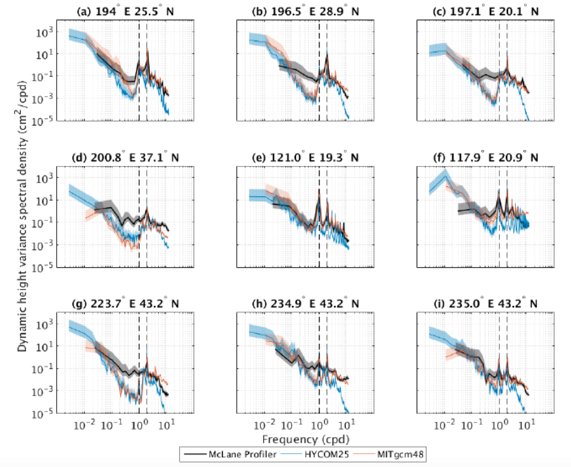
Our group has been comparing the IGW spectrum in the HYCOM and MITgcm simulations with theoretical predictions and with a variety of observations. The 1/12°, 1/24°, and 1/48° MITgcm simulations are referred to as MITgcm12, MITgcm24, and MITgcm48 in the plots below, while the 1/12.5° and 1/25° HYCOM simulations are referred to as HYCOM12 and HYCOM25. The MITgcm simulations have 90 z-levels in the vertical direction, while the HYCOM simulations have 41 hybrid layers in the vertical direction. In Figure 1, taken from a paper in revision (Savage et al.), we compare the dynamic height variance frequency spectra in HYCOM and MITgcm simulations and 9 in-situ McLane vertical profilers in the Pacific Ocean. The processed McLane profiler data is at both high vertical resolution (2 decibars) and high temporal resolution (one hour), and is therefore well suited for the computation of high-frequency dynamic height variance. The MITgcm supertidal variance lies closer to the observed variance than the HYCOM variance does, probably because of the higher horizontal and vertical resolution.

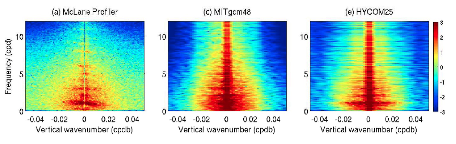
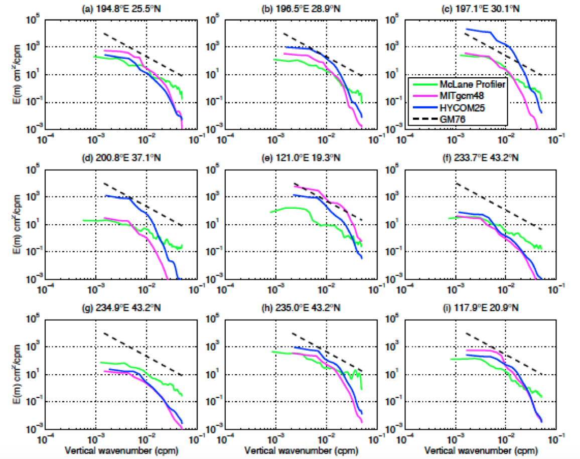
In Figure 2, taken from another paper in preparation (Ansong et al.), the frequency-vertical wavenumber spectra of horizontal kinetic energy in MITgcm48 and HYCOM25 simulations are compared to spectra computed from McLane profiler data at a location in the Pacific Ocean. The near-symmetry about the x-axis implies nearly equal amounts of upward- and downward-propagating energy, in agreement with longstanding ideas about the IGW continuum [Garrett and Munk, 1975]. In Figure 3, the frequency-vertical wavenumber spectra at 9 Pacific Ocean locations are integrated over frequency to yield vertical wavenumber spectra. The McLane spectra generally follow the Garrett and Munk [1975] m^-2 prediction over nearly 2 decades. The models follow the predicted slope over some low wavenumbers, but roll off more steeply at higher vertical wavenumbers, due to inadequate model resolution.

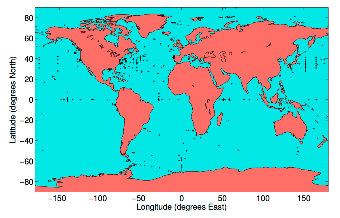
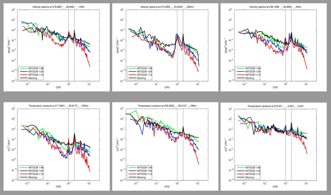
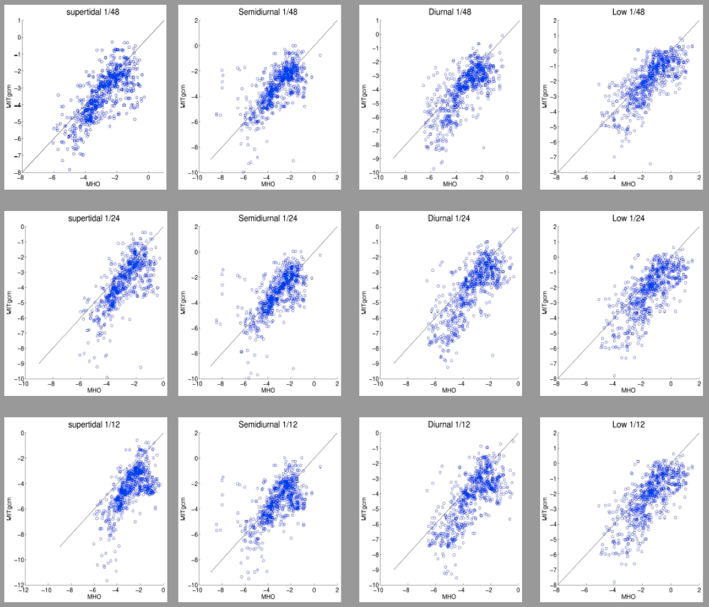
We have McLane profiler data, suitable for the IGW comparisons described above, at only 9 locations. We are also testing the models over a wide range of frequencies using historical moored observations of velocity variance (kinetic energy) and temperature variance to test the models over a range of frequencies [Luecke et al., in preparation]. The historical observations do not have the high vertical resolution of the McLane profiler observations, but are available at more than 1000 locations throughout the globe, as seen in Figure 4. Figure 5 shows example frequency spectra of velocity variance (kinetic energy) and temperature variance in the MITgcm compared to observations. At supertidal frequencies, the MITgcm spectra compare more closely with observations as model resolution increases. In Figure 6, we display scatterplots of temperature variance, integrated over low frequencies, semidiurnal frequencies, diurnal frequencies, and supertidal frequencies, from MITgcm12, MITgcm24, and MITgcm48, versus the variance of historical observations. While model resolution changes the temperature variance in other bands, its largest effect is seen at supertidal frequencies. The temperature variance of MITgcm48 compares best with that of the observations, in that the points display the least amount of bias with respect to the one-to-one line.

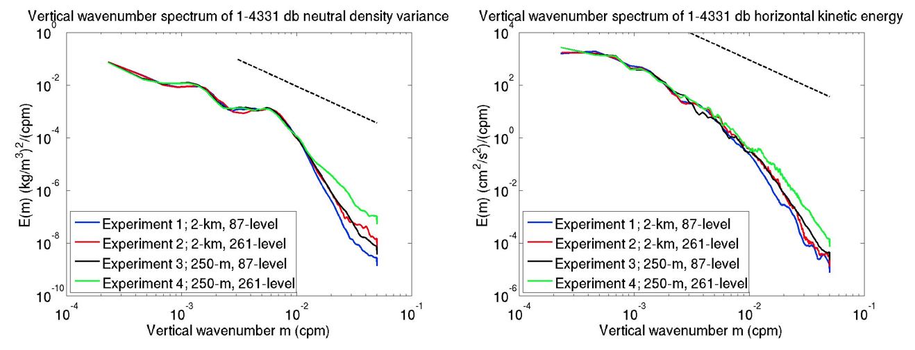
In Figure 7, we examine the impact of increasing horizontal and vertical resolution on even-higher-resolution regional simulations that are forced at their boundaries by the global MITgcm48 simulation. The regional simulations include a simulation with horizontal grid spacing (2 km) and vertical grid spacing (87 z-levels) equal to that of the global model, and simulations with higher horizontal resolution (250 m grid spacing), higher vertical resolution (261 z-levels), or both. Figure 7 shows the vertical wavenumber spectra of high-frequency (periods < 2 days) neutral density and horizontal kinetic energy. The vertical wavenumber spectra flattens out (increases in strength) at the high-vertical-wavenumber end in response to an increase in either horizontal or vertical resolution, and increases even more when both horizontal and vertical resolution are increased. The high horizontal and vertical resolution simulation lies closest to the Garrett and Munk [1975] m^-2 prediction. The vertical wavenumber spectra are of particular interest for understanding ocean mixing, because the Richardson number criterion for Kelvin-Helmholtz shear instability depends on the vertical derivative of velocity, and the vertical derivative of a wave field with vertical wavenumber m is proportional to m.

Summary and Other Work

We are comparing the global HYCOM and MITgcm simulations to a variety of in-situ datasets. Modeled frequency spectra of dynamic height variance, frequency-vertical wavenumber spectra of horizontal kinetic energy, and vertical wavenumber spectra of neutral density variance and horizontal kinetic energy, are compared with spectra computed from McLane profiler data, which offers high vertical and temporal resolution data of velocity, temperature, and salinity. However, McLane data suitable for such computations is only available at 9 locations in the Pacific Ocean. A quasi-global comparison is being done with historical moored observations of temperature and velocity, which offer more than 1000 measurement locations, at the cost of a large loss in vertical resolution. In all of the model-data comparisons, a consistent theme is the importance of higher model resolution. Consistent with this, we are finding that increasing either horizontal or vertical resolution, in regional simulations done with very fine grid spacing, moves vertical wavenumber spectra of neutral density variance and horizontal kinetic energy closer to theoretical predictions.

We are using the HYCOM and MITgcm simulations to study the horizontal wavenumber-frequency spectra of surface ocean horizontal kinetic energy and SSH variance in several regions, as a function of model resolution. Consistent with our earlier work in Richman et al. [2012], we find that high-frequency motions can dominate the high-wavenumber end of the SSH variance wavenumber spectrum, with consequent implications for the SWOT mission. We are also using the models to study the nonlinear interactions that underlie the IGW spectrum, and to study ocean mixing.

References

Ansong, J.K., B.K. Arbic, M.H. Alford, M.C. Buijsman, J.F. Shriver, Z. Zhao, J.G. Richman, H.L. Simmons, P.G. Timko, A.J. Wallcraft, and L. Zamudio (2017), Semidiurnal internal tide energy fluxes and their variability in a Global Ocean Model and moored observations, J. Geophys. Res. Oceans, 122, 1882–1900, doi:10.1002/2016JC012184.

Arbic, B.K., S.T. Garner, R.W. Hallberg, and H.L. Simmons (2004), The accuracy of surface elevations in forward global barotropic and baroclinic tide models, Deep Sea Res., Part II, 51, 3069–3101, doi:10.1016/j.dsr2.2004.09.014.

Arbic, B.K., A.J. Wallcraft, and E.J. Metzger (2010), Concurrent simulation of the eddying general circulation and tides in a Global Ocean Model, Ocean Modell., 32, 175–187.

Buijsman, M.C., B.K. Arbic, J.G. Richman, J.F. Shriver, A.J. Wallcraft, and L. Zamudio (2017), Semidiurnal internal tide incoherence in the equatorial Pacific, J. Geophys. Res., in press.

Chassignet, E.P., and X. Xu (2017), Impact of horizontal resolution (1/12° to 1/50°) on Gulf Stream separation, penetration, and variability, J. Phys. Oceanogr., in press.

Cummings, J.A., and O.M. Smedstad (2013), Variational data assimilation for the global ocean, in Data Assimilation for Atmospheric, Oceanic and Hydrologic Applications (Vol. II), S.K. Park and L. Xu (eds.), DOI 10.1007/978-3-642-35088-7_13, 303-343.

D'Asaro, E. A. (1984), Wind forced internal waves in the North Pacific and Sargasso Sea, J. Phys. Oceanogr., 14, 781–794.

Dushaw, B.D., B.D. Cornuelle, P.F. Worcester, B.M. Howe, D.S. Luther, D.S. (1995), Barotropic and baroclinic tides in the central North Pacific Ocean determined from long-range reciprocal acoustic transmissions, J. Phys. Oceanogr. 25, 631–647.

Egbert, G.D., A.F. Bennett, and M.G.G. Foreman (1994), TOPEX/POSEIDON tides estimated using a global inverse model, J. Geophys. Res., 99, 24,821–24,852.

Garrett, C.J.R., and W.H. Munk (1975), Space-time scales of internal waves. A progress report, J. Geophys. Res., 80, 291–297, doi:10.1029/JC080i003p00291.

Le Traon, P.Y., P. Klein, B.L. Hua, and G. Dibarboure (2008), Do altimeter wavenumber spectra agree with the interior or surface quasigeostrophic theory?, J. Phys. Oceanogr., 38, 1137–1142, doi:10.1175/ 2007JPO3806.1.

Müller, M., B.K. Arbic, J.G. Richman, J.F. Shriver, E.L. Kunze, R.B. Scott, A.J. Wallcraft, and L. Zamudio (2015), Toward an internal gravity wave spectrum in global ocean models, Geophys. Res. Lett., 42, 3474–3481, doi:10.1002/2015GL063365.

Müller, P., G. Holloway, F. Henyey, and N. Pomphrey (1986), Nonlinear interactions among internal gravity waves, Rev. Geophys, 24(3), 493–536, doi:10.1029/RG024i003p00493.

Ngodock, H.E., I. Souopgui, A.J. Wallcraft, J.G. Richman, J.F. Shriver, and B.K. Arbic (2016), On improving the accuracy of the M2 barotropic tides embedded in a high-resolution global ocean circulation model, Ocean Modell., 97, 16–26, doi:10.1016/j.ocemod.2015.10.011.

Ray, R.D., and D.A. Byrne (2010), Bottom pressure tides along a line in the southeast Atlantic Ocean and comparisons with satellite altimetry, Ocean Dyn., 60, 1167–1176.

Ray, R.D., and G.T. Mitchum (1996), Surface manifestation of internal tides generated near Hawaii, Geophys. Res. Lett. 23, 2101–2104.

Richman, J.G., B.K. Arbic, J.F. Shriver, E.J. Metzger, and A.J. Wallcraft (2012), Inferring dynamics from the wavenumber spectra of an eddying global ocean model with embedded tides. Journal of Geophysical Research 117, C12012, doi:10.1029/2012JC008364.

Rocha, C.B., T.K. Chereskin, S.T. Gille, and D. Menemenlis (2016), Mesoscale to submesoscale wavenumber spectra in Drake Passage, J. Phys. Oceanogr., 46, 601–620, doi:10.1175/JPO-D-15-0087.1.

Sasaki, H., and P. Klein (2012), SSH wavenumber spectra in the North Pacific from a high-resolution realistic simulation, J. Phys. Oceanogr., 42, 1233–1241, doi:10.1175/JPO-D-11-0180.1.

Shriver, J.F., J.G. Richman, and B.K. Arbic (2014), How stationary are the internal tides in a high-resolution global ocean circulation model?, J. Geophys. Res. Oceans, 119, 2769–2787, doi:10.1002/2013JC009423.

Wunsch, C. (1975), Internal tides in the ocean, Rev. Geophys. Space Phys., 13, 167–182.

Simmons, H.L., R.W. Hallberg, and B.K. Arbic (2004), Internal wave generation in a global baroclinic tide model, Deep Sea Res., Part II, 51, 3043–3068.

Zhao, Z., M.H. Alford, J.B. Girton, L. Rainville, and H. L. Simmons (2016), Global observations of open-ocean mode-1 M2 internal tides, J. Phys. Oceanogr., 46, 1657–1684, doi:10.1175/JPO-D-15-0105.1.