Documents
OSIRIS: Ocean, Sea-ice and Rain Investigations for SWOT
A UK-wide programme of research in preparation for SWOT
PI: Francesco Nencioli (PML - Plymouth, UK)
Co-PIs: Steve Baker (CPOM, UCL - London, UK), Chris Hughes (UoL - Liverpool, UK), Adrian Martin (NOCS - Southampton, UK), Graham Quartly (PML - Plymouth, UK), Andrew Shepherd (CPOM - University of Leeds, UK), Chris Wilson (NOCL - Liverpool, UK)
1. Introduction
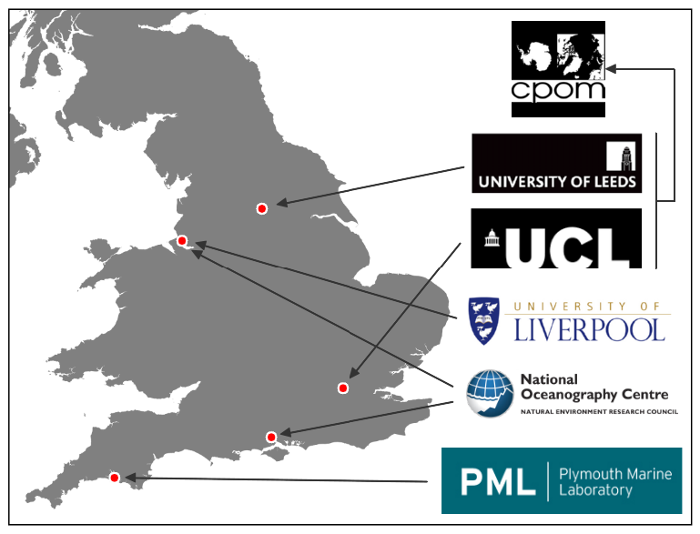
The OSIRIS project brings together the work plans of seven investigators from five UK organizations, including University of Liverpool (UoL), the National Oceanography Centre, Southampton and Liverpool (NOCS and NOCL, respectively), Plymouth Marine Laboratory (PML) and the Centre for Polar Observations and Modelling (CPOM). The consortium gathers a broad range of UK expertises which will contribute to different aspects of SWOT research priorities for oceanography and cryosphere.
OSIRIS activities consist of a series of independent studies developed by the various groups within the consortium. These studies cover open ocean and coastal oceanography, as well as sea-ice and atmospheric effects on instrumental performance. They are based on the development of new analysis techniques and methodologies from examination of model output and improvements to modelling, or through the construction of datasets and climatologies based on currently available satellite data.
2. Objectives and Approach
These activities can be structured into 3 main categories, each comprising of one or more work packages (WP) associated with a defined objective:
- High-resolution numerical models: open ocean processes:
- WP1: Investigate (sub)mesoscale dynamics in ocean models
- WP1.1: Small-scale eddies and eddy mean-flow interactions. We will investigate scales at 200 km or shorter which are barely resolved in present altimeter products. These include the generation of "modons" (i.e. self- advecting eddy pairs analogous to smoke rings). We will focus on how steep topography affects their propagation as well as eddy-mean flow energy exchange.
- WP1.2: Constrained stochastic eddy parametrization for ocean models. We will develop stochastic parametrisation for realistic ocean models, guided by observed frequency-wavenumber spectra, in order to improve simulation of large- scale climate. Analysis of the wavenumber spectra produced by the SWOT simulator will help in assessing the expected contribution of SWOT observations in the development of such parametrizations.
- WP1.3: Mesoscale to sub-mesoscale dynamics, transport and mixing. Lagrangian coherent structures (LCS) will be used to investigate mechanisms of transport and mixing. These will be calculated from a) full simulation, b) resampling similar to traditional altimetry and c) SWOT simulator for a detailed inter- comparison and to evaluate the robustness of LCS analysis to SWOT-like sampling and errors.
- WP1: Investigate (sub)mesoscale dynamics in ocean models
- Satellite data: coastal ocean, in-situ & biophysical interactions:
- WP2: Link open ocean and coastal altimetry observations. The main aim is to bridge the gap between altimetry measurements (limited within 10 km to the coast) and tide-gauge measurements. Models and current altimeter observations will be used to identify the main coastal processes within such a gap which determine sea level and dynamic topography at the coast. Analysis based on the SWOT simulator will allow us to assess the capabilities of the SWOT mission to recover the relevant scales.
- WP3: Optimize (sub)mesoscale in-situ sampling strategies. We will further develop satellite-based diagnostics for the near-real time optimization of (sub)mesoscale oriented field experiments. New Sentinel 2 and 3 observations will be included to support future campaigns within the SWOT mission.
- WP4: Investigate biophysical interactions at the (sub)mesoscale. The dynamics of physical-biogeochemical interactions will be investigated in regions of intense mesoscale stirring combining remote sensing and in-situ observations. We will focus on the role of frontogenesis in leading to stronger vertical circulation and increased primary productivity, and we will assess SWOT capabilities in improving our ability to diagnose frontogenesis and its influence on production.
- Effects on instrumental performance:
- WP5: Evaluate potential for sea-ice observations and modelling. Analysis of existing altimeter data (Cryosat-2, AltiKa, Sentinel-3) over land-and sea- ice will be used to monitor changes in Arctic glaciers (sea-ice thickness, ice-sheet elevation change, dynamic ocean topography). We will improve the classification and retracking of waveforms to identify reflections from sea-ice or snow layers on top of that, setting the framework to interpret SWOT data in those regions and assess their potential to provide essential climate variables (ECV's).
- WP6: Evaluate wind and rain effects on reflected Ka-band signal. The accuracy of SWOT measurements will be affected by the strength of the return signal, which in open ocean regions is mainly affected by wind and rain. Their effect will be analysed based on AltiKa observations, providing the range of values to be expected for backscatter strength and how rapidly they change with distance. This will help design a wind speed algorithm for SWOT and demonstrate how the spatial scales of variation due to rain will affect the modelling of radar returns.
3. Analysis and Anticipated Results
Up to date, the major results from the consortium activities have been obtained for WP1.2, WP2 and WP6.
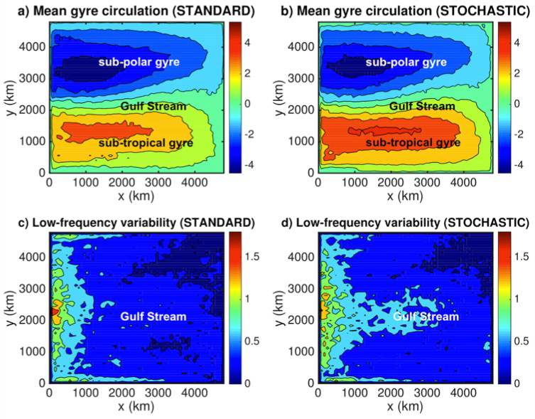
WP1.2: Constrained Stochastic Eddy Parametrization for Ocean Models (C. Wilson)
Two idealised simulations of the North Atlantic circulation with the Q-GCM model. 10-year mean surface dynamic pressure (m2s-2) for: a) the control run b) a run with spatially uncorrelated AR(1) forcing of pressure. Standard deviation of the pressure (m2s-2) filtered to include only low- frequency variability greater than 180 for c) the control run, d) the AR(1) forced run.
The forcing is able to generate low-frequency variability in the Gulf Stream region and also intensify the subtropical gyre. SWOT observations will add extra information to the frequency-wavenumber spectrum, which may then be used to constrain the stochastic forcing.
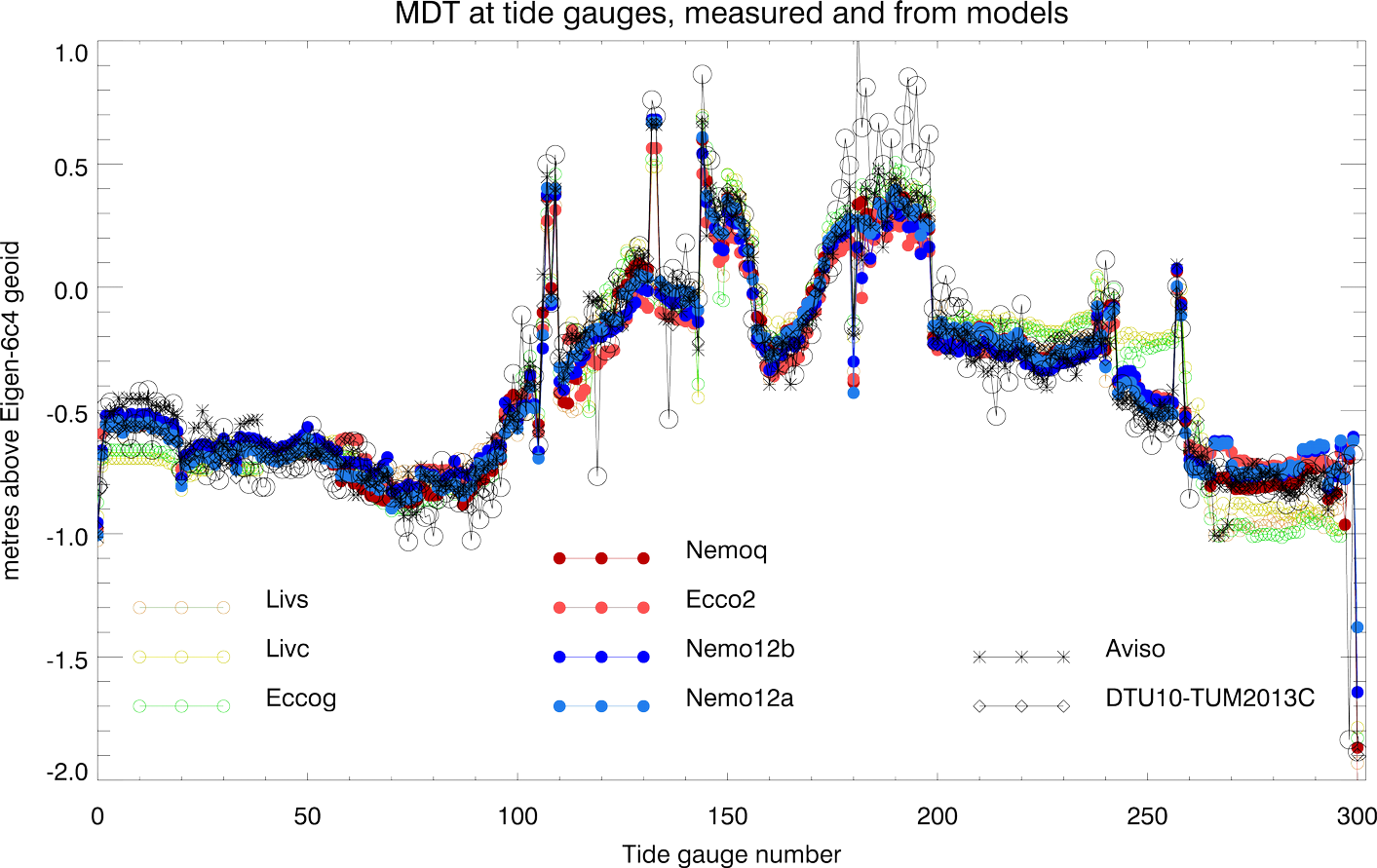
WP2: Link Open Ocean and Coastal Altimetry Observations (C. Hughes)
As part of an ESA-funded programme (GOCE++ Dycot), data have been gathered from 301 tide gauges around the world that have known GPS ties. The figure shows the 2003-2007 (inclusive) mean dynamic topography computed from these values, in combination with the Eigen-6c4 geoid up to degree and order 2190. Black circles show these dynamic topography values, together with the equivalent values from a series of ocean models (colours) and altimetry-based dynamic topographies (other black symbols). The tide gauges are ordered approximately following the world coastline: Northern Russia, Europe, Africa, the Indian Ocean, East Asia, Indonesia, Australia and New Zealand, Pacific Islands, Pacific Americas north to south, Atlantic Americas south to north, Antarctica (one point).
The agreement with coarse resolution models (1 degree resolution; open symbols) is notably worse than with finer- resolution (1/4 to 1/12 degree), as is particularly clear in the western North Atlantic region (approximately gauges 230 to 295). The tide gauge results show a systematic difference from models on tropical Pacific islands (178-200), tentatively identified as an effect of the unresolved and similar geoid structure associated with these sites. We also find (not shown) that the in situ gravity contribution to the geoid is crucial, with much worse agreement using only the resolution achievable with satellite gravity.
This first stage of work will be extended by considering how and where coastal altimetry can be used to improve the measurement of coastal sea level, and reduce the impact of the smallest resolution features in the geoid.
WP6: Evaluate Wind and Rain Effects on Reflected Ka-band Signal (G. Quartly)
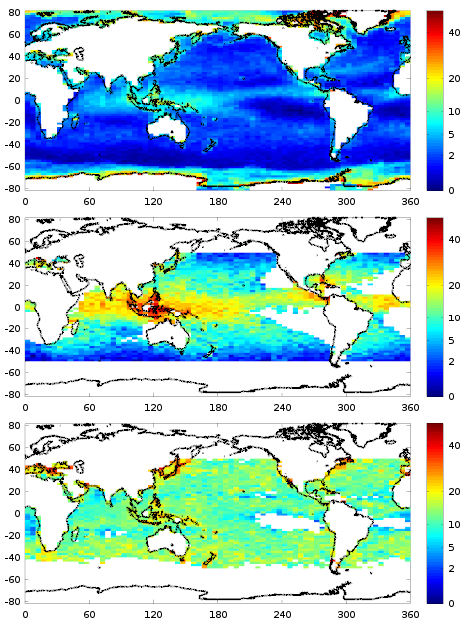
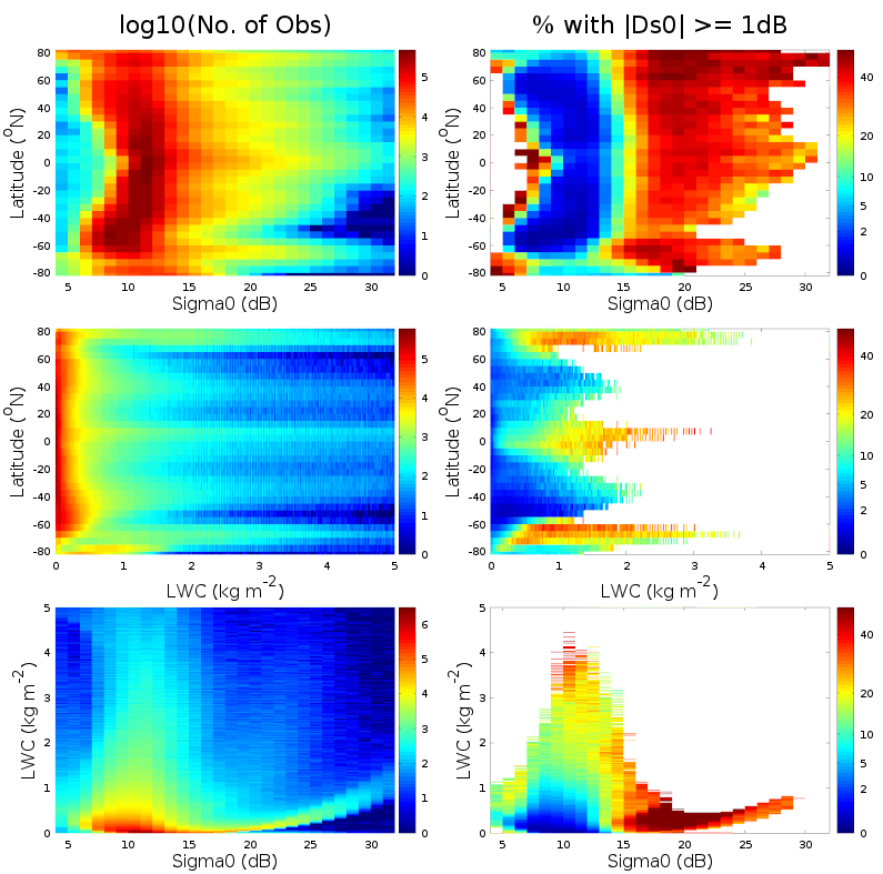
We have considered 2 years of AltiKa data (Jan 2014-Jan 2016) and looked at the frequency of steps of 1dB (positive or negative) between 2 consecutive 1Hz records. This means the average footprint considered here is smeared over 7km along track, with the records 7 km apart. The percentage of step changes exceeding 1 dB is shown in the top plot of the first figure (note the use for a non-linear colour scale to show how low the occurrence is in many regions). There are 4 main likely causes -- i) Rain (providing strong attenuation), ii) Ice (either icebergs giving bright reflections or leads within Arctic sea-ice providing a near-glassy surface), iii) Slicks (either biogenic or mineral oil causing very flat conditions, possibly associated with "sigma0 blooms") & iv) Small-scale wind variability in very calm conditions.
A consideration of the local conditions is shown in the 2nd figure, with sigma0 being backscatter strength [median value=11.2 dB, and 10th & 90th percentiles being 9.2 & 13.2 dB, representing highest and lowest winds respectively] & LWC=radiometer-derived Liquid Water Content, denoting excessive moisture in the air, as a likely indicator of rain. High LWC values at high latitudes are probably due to ice rather than atmospheric moisture.
Using this contextual information, we define rain-likely conditions as LWC>=0.4 AND -50<= lat <= 50. The second plot in the first figure shows the probability of steps in sigma0 exceeding 1 dB in these conditions. The 3rd plot in that figure is for calm conditions (LWC<0.1 AND -50<= lat <= 50 AND sigma0>13.2). This will include 1dB steps dues to slicks or small-scale wind variability.
The analysis will be repeated using the 40Hz data, thus with smaller real instrument footprint, and permitting step changes to be examined at a scale of 1.5-2km (i.e. the limitation of the field-of-view).