Documents
SWOT and the Ice Covered Oceans of the Arctic and Antarctic: Sea Surface Height and Sea Ice Freeboard
R. Kwok and T.W.K. Armitage (Jet Propulsion Laboratory, California Institute of Technology Pasadena - California USA)
1. Introduction/Objectives
This project addresses research opportunities offered by the SWOT mission that pertain to observations of sea surface height and sea ice freeboard/thickness of the ice- covered oceans. Since the effects of clouds (which plague lidar measurements especially during the summer) are negligible in radar data, the SWOT mission will be capable of providing year-round measurements of sea and ice surface heights. Even though the sampling of sea surface of the polar oceans of the Northern and Southern Hemispheres is limited to only a few percent of the area of exposed ocean within bounds of a satellite's inclination, the SWOT resolution will allow uninterrupted coverage of the sea surface through the openings/fractures in the ice cover for determination of dynamic topography and calculations of sea ice freeboard.
The objective then is to understand the feasibility and utility of SWOT data for providing sea and ice surface height measurements over the ice-covered oceans, and more specifically to investigate special procedures required to separate returns from the ocean and sea ice surfaces, to assess the effects of penetration into the snow layer on freeboard calculations and in particular, the achievable accuracy of sea surface heights and freeboard elevations. AirSWOT acquisitions over sea ice or snow targets, if available, will be used for understanding the expected quality of SWOT retrievals for sea ice work. A secondary objective is to support the definition of the measurement requirements and data parameters required for the ice-covered oceans.
2. Approach
Below, we describe briefly the general retrieval approaches and the application to SWOT.
2.1 Retrieval of Freeboard, Ice Thickness, and SWOT
Assuming isostatic equilibrium, ice thickness (hi) is calculated with the following equation:
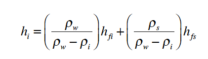
hfi and hfs are sea ice freeboard and snow depth, and Ρw, Ρi, and Ρs are the bulk densities of water, ice, and snow. The relationship between freeboard, thickness, and ice draft is shown in Fig. 1. Recent work demonstrated the efficacy of obtaining large-scale thickness estimates using the retrieved freeboard from profiling lidars and radars [e.g., Kwok et al., 2009; Laxon et al., 2013; Kwok and Cunningham, 2015].

SWOT's synthetic aperture radar interferometry offers advancements over the lidar altimetry in two respects: (1) the microwave wavelength is relatively unaffected by cloud cover and (2) it provides swath coverage (120 km) instead of along-track height profiles. Clouds limit lidar sampling of the ice-covered oceans and the coverage issue is especially acute during the summer and near the ice edge where strong atmosphere-ice-ocean interactions take place. Due to clouds, lidar coverage of the polar oceans is reduced to less than ~40% of the Arctic Ocean after the onset of spring melt (from almost 90% during the winter), and the degradation in coverage is even higher near the ice edge. With SWOT, the uninterrupted all-season coverage of the polar oceans represents a significant advantage to the sampling of changes in ice thickness associated with summer and fall processes not observed by lidars. In addition, the fine spatial resolution and swath coverage of the SWOT interferometer are advancements over the synthetic aperture radar mode of the CryoSat-2 altimeter (resolution: 1.5 km by 300m) [Wingham, 2005]. And, fine spatial resolution in radar altimetry is important for resolving small areas of open water (leads, melt ponds) within the sea ice cover. Furthermore, the total swath width of 120 km—achieved by looking at both sides of the nadir track—would allow two- dimensional depictions of the spatial variability of the freeboard/thickness of the ice cover that are important for quantifying exchanges of momentum between sea ice and the atmosphere and ocean.
The selected SWOT orbit coverage extends from 78°S to 78°N with a 22-day repeat period. Even though this provides only partial coverage of the Arctic Ocean, the instrument covers the entire Southern Ocean sea ice cover. With the scientific benefits discussed above, the SWOT instrument is poised to provide unique contributions to polar science. As mentioned earlier, the convergence of orbits in the polar-regions at lower polar latitudes increases the spatial density and frequency of observations of SSH from the high-Arctic to the ice margins of the Arctic, where the largest changes in the Arctic are taking place.
Given our experience with ICESat, the challenges to develop the algorithms for retrieval of sea ice freeboard and thickness from SWOT elevation estimates include: 1) developing procedures for ice/water discrimination; 2) developing procedures for identification of elevations in narrow leads; and 3) understanding the impact of sub- surface returns from snow (due to penetration at Ka-band) on retrieval of surface elevation.
As mentioned earlier, there are two leading topics of importance in considering the use of SWOT data for determination of sea surface height and sea ice freeboard. The first is our ability to separate the sea surface returns in open-water leads from the ice returns within the ice cover, and the second is our understanding of the depth of penetration of the Ka-band radar (in this case, the interferometric range) into the snow volume over sea ice. The former pertains to the sampling of the sea and ice surfaces provided by SWOT instrument; the latter impacts our computation of freeboard, as uncertainties in freeboard and snow depth propagate into estimates of thickness and volume.
2.2 Ice/Water Discrimination in SWOT

The identification of open water depends on the scattering contrast between ice and open water leads at near-nadir look angles (SWOT look angles are up to 4.5°). Quasi-specular returns in CryoSat-2 (Ku-band altimeter) have been used successfully for separating open water or thin ice returns in leads from the diffuse returns from sea ice. Since there is a steep drop in backscatter at off-nadir incidence angles, the question is whether there would be sufficient contrast between open water and sea ice in SWOT returns for effective discrimination of the two surfaces. In addition to radar backscatter, there are also other interferometric parameters (e.g., i correlation = ‹v1 , v2*›) that may be of use for the separation of smooth water surfaces from rougher ice surfaces but there are other considerations involved.
Another topic that is unique to SWOT is that an aggregate number of radar samples are required to provide an accurate sea surface reference for freeboard calculations. Since leads are long and narrow openings, one question is whether there are leads that are wide enough and long enough to provide the number of samples needed for accurate surface height estimation. Fig. 2shows the lead width distribution compared to an ICESat footprint of 70 m. Even though 80% of Arctic leads are less than 70 m wide, a sufficient number of leads seen in ICESat were available to provide sea surface references for basin-scale estimates of sea ice freeboard [Kwok et al., 2009]. In any case, the question is how to optimally aggregate sea ice leads within a SWOT swath for the purposes of freeboard calculations and ice thickness estimation.
2.3 Penetration into the Snow Layer
Due to the density differences between snow and ice, the height of the exact snow-freeboard or ice-freeboard is required for the computation of sea ice thickness using the assumption of hydrostatic equilibrium (see equation above). Respectively, the two freeboards are the height of the air-snow (a-s) interface and snow-ice (s-i) interfaces above the local sea surface (see Fig. 1). The lidar returns from ICESat (1064 nm lidar) are expected to be from the a-s surface because there is negligible penetration at that wavelength into the snow layer, while the radar returns from CryoSat-2 (Ku-band altimeter) are generally expected to be from the s-i interface. The penetration depth of Ka- band over dry snow pack is in the range of 0.1-0.3 m (compared to 2-10 m at Ku-band).
Since Arctic snow depth in winter is within the range of 0.1-0.3 m, the penetration issue could be a factor if potential subsurface returns were not considered in freeboard calculations. There are also potential differences between the estimated heights obtained from traditional altimetry and interferometry (in the presence of volume scattering). We will to investigate these issues further as part of this project.
3. Analysis and Anticipated Results
Anticipated results are as follows:
- Simulations of SWOT returns over the Arctic sea ice cover.
- Feasibility and expected accuracy of freeboard and sea surface height estimates within the ice-covered oceans.
- Definition of necessary SWOT parameters for derivation of freeboard and sea surface height.
- Definition of area for post-launch validation of SWOT estimates.
4. References
Kwok, R., and G.F. Cunningham (2015), Variability of Arctic sea ice thickness and volume from CryoSat-2, Phil. Trans. R. Soc. A, 373(2045), doi:10.1098/rsta.2014.0157.
Kwok, R., G.F. Cunningham, M. Wensnahan, I. Rigor, H.J. Zwally, and D. Yi (2009), Thinning and volume loss of the Arctic Ocean sea ice cover: 2003–2008, J. Geophys. Res., 114(C7), doi:10.1029/2009jc005312.
Laxon, S.W., et al. (2013), CryoSat-2 estimates of Arctic sea ice thickness and volume, Geophys. Res. Lett., 40(4), 732-737, doi:10.1002/grl.50193.
Wingham, D. (2005), CryoSat: A mission to the ice fields of Earth, Esa Bulletin- European Space Agency (122), 10-17.